Fertility prediction using LISS data

Last updated on 2024-07-02 | Edit this page

Estimated time: 300 minutes

Overview

Questions

How do you start a real-world machine learning project?

Objectives

Be able to successfully start a real-world machine learning project.

Introducing the assignment

In this assignment you will work individually on a machine learning problem. The end-goal is that you are able to pick up a real-world machine learning project.

This assignment will guide you through such a real-world project.

A note on how to learn the most from this assignment

Some participants will learn the most from just loading in the data, explore and build a machine learning pipeline and solve all problems you encounter on the way yourself. Most of you will likely need the guidance of the exercises and solutions in this assignment to bring you up to speed. Try to take some time to solve the challenges yourself before looking at the solutions. But if you get stuck for too long do not hesitate to let the solutions guide you, or ask one of the trainers.

You will have to find a balance between guidance and self-exploration yourself.

1. Introducing the problem

The goal is to predict who will have a child in the next 3 years, based on all the data from previous years.

To train your models, you will have all the background data (features) up to 2020 and the data about the outcome - having a child in 2021-2023. So, the outcome is binary (0 - no new children in 2021-2023, 1- at least one new child in 2021-2023). The performance of the models will then be tested on the remaining cases.

You are encouraged to use different strategies to predict the outcome – e.g. theory-driven (to select a relatively small set of variables that were found significant in previous studies) and data-driven (e.g. features selected based on regularisation).

Features that can be used for the first simple models: gender, age, education level, current partnership status, health, religion, fertility intentions

Challenge: Formulating the problem

What kind of problem is this? Classification or regression?
What are the inputs (features) and what are the outcomes (target)?
How many classes are there in the target variable?

Show me the solution

This is a classification problem
Inputs are the background data of the persons (for example gender, age, partnership status), outcome is who will have a child in the next 3 years.
There are 2 classes: not having a child in the next 3 years (0) and having a child in the next 3 years (1). This is thus a binary classification problem.

2. Reading in and exploring the data

Challenge: Reading in the data

Try to read in the data using pandas. The features are in ‘PreFer_train_data_only_2020_vars.csv’, the outcome variable is stored in ‘PreFer_train_outcome.csv’/ Hint: You might run into an encoding error. See if you can fix it by googling for a solution.

Show me the solution

Reading in the features:

PYTHON

# This might result in UnicodeDecodeError: 'utf-8' codec can't decode byte 0x92 in position 50416: invalid start byte
data = pd.read_csv('data/PreFer_train_data_only_2020_vars.csv')

# To tackle the encoding error:
data = pd.read_csv('data/PreFer_train_data_only_2020_vars.csv', encoding='cp1252')

Reading the outcomes:

PYTHON

outcome = pd.read_csv('data/PreFer_train_outcome.csv')

Challenge: Exploring the data

Explore the data.

How many features do we have?
How many samples do we have?
Are the outcome and features datasets ordered in the same way?
What type of data do we have as features?
Is the target variable well balanced?
Do we have any missing data?

Show me the solution

Quickly explore the data:

PYTHON

data.shape

OUTPUT

(6418, 2291)

PYTHON

data.head(10)

	nomem_encr	cf20m_m	cf20m001	cf20m002	cf20m003	cf20m004	cf20m005	cf20m007	cf20m008	cf20m009	...	nettohh_f_2020	nettoink_2020	nettoink_f_2020	oplcat_2020	oplmet_2020	oplzon_2020	partner_2020	sted_2020	woning_2020	woonvorm_2020
0	712619	NaN	NaN	NaN	NaN	NaN	NaN	NaN	NaN	NaN	...	NaN	NaN	NaN	NaN	NaN	NaN	NaN	NaN	NaN	NaN
1	706448	NaN	NaN	NaN	NaN	NaN	NaN	NaN	NaN	NaN	...	3263.0	1251.0	1251.0	3.0	3.0	3.0	1.0	1.0	1.0	3.0
2	729145	202009.0	2.0	2009.0	1.0	45.0	1939.0	1.0	NaN	1945.0	...	8500.0	4250.0	4250.0	6.0	6.0	6.0	1.0	1.0	1.0	3.0
3	729424	NaN	NaN	NaN	NaN	NaN	NaN	NaN	NaN	NaN	...	NaN	NaN	NaN	NaN	NaN	NaN	NaN	NaN	NaN	NaN
4	715619	202009.0	16.0	NaN	1.0	30.0	1964.0	1.0	NaN	1954.0	...	NaN	NaN	NaN	4.0	4.0	5.0	1.0	3.0	1.0	2.0
5	715353	NaN	NaN	NaN	NaN	NaN	NaN	NaN	NaN	NaN	...	NaN	NaN	NaN	NaN	NaN	NaN	NaN	NaN	NaN	NaN
6	704754	NaN	NaN	NaN	NaN	NaN	NaN	NaN	NaN	NaN	...	NaN	NaN	NaN	NaN	NaN	NaN	NaN	NaN	NaN	NaN
7	726292	NaN	NaN	NaN	NaN	NaN	NaN	NaN	NaN	NaN	...	NaN	NaN	NaN	NaN	NaN	NaN	NaN	NaN	NaN	NaN
8	716711	202009.0	16.0	NaN	2.0	31.0	1950.0	1.0	NaN	1949.0	...	4166.0	2166.0	2166.0	5.0	5.0	5.0	1.0	2.0	1.0	2.0
9	729919	NaN	NaN	NaN	NaN	NaN	NaN	NaN	NaN	NaN	...	NaN

PYTHON

outcome.head(10)

	nomem_encr	new_child
0	712619	NaN
1	706448	NaN
2	729145	NaN
3	729424	NaN
4	715619	0.0
5	715353	NaN
6	704754	NaN
7	726292	NaN
8	716711	1.0
9	729919	NaN

There are 2290 features (excluding nomem_encr which is just an identifier)
There are 6418 samples
The outcome and features seem to be ordered in the same way
The features are both categorical and numerical

PYTHON

outcome['new_child'].describe()

OUTPUT

count    987.000000
mean       0.214792
std        0.410886
min        0.000000
25%        0.000000
50%        0.000000
75%        0.000000
max        1.000000
Name: new_child, dtype: float64

The target variable is pretty unbalanced, only 21.5 % of the samples are in the 1 class
There are is a lot of missing data in the features as well is in the output.

3. Taking a step back

Before you start enthusiastically typing all kinds of pandas and sklearn commands that you just learned. Now that you have explored the data, it is good to take a step back and think about how you want to approach the problem.

Challenge: What steps to take next?

Now that you know the data a little bit. What are the steps that you need to take before we can train our first modeling pipeline. Think about the essential steps that will get you a working pipeline. Take shortcuts where possible. It does not need to be a very accurate predictor (yet ;) ). Also think about the order in which to do things.

NB: You do not have to execute the steps yet, in the next challenges we will guide you through the steps one-by-one.

Show me the solution

These are the minimum steps that need to happen, in this order (the order is a bit arbitrary, it is important that you split the data before doing any fitting):

Remove samples that have a missing outcome variable
Select features
Deal with missing data. The quickest way is to just drop all rows that have any missing value.
Split the data in a train and test set.
Preprocess the features: scaling for numerical values, one-hot encoding for categorical values.
Train the model and evaluate!

We will not worry about the unbalanced target yet. Let’s first see how a model performs on the unbalanced dataset.

4. Prepare the data

Challenge: Remove samples with a missing outcome

For a majority of the samples we have a missing outcome value. Can you remove those samples from the dataset? How many samples do we have left?

Note: To drop people with missing outcome from the training data, the variable “outcome_available” should be used. That iss because the function for preprocessing that you will need to edit for real submissions (’’clean_df” function) does not take the holdout_outcome dataset as an argument (to prevent cheating e.g. creating a column with predictions which equals the real outcome from the holdout data).

Show me the solution

PYTHON

y_missing = data['outcome_available'] == 0

# Drop samples in both `data` and `outcome`:
data = data.drop(data[y_missing].index, axis='rows')
outcome = outcome.drop(outcome[y_missing].index, axis='rows')
outcome.shape

OUTPUT

(987, 2)

We have 987 samples left

Challenge: Selecting data for a quick and dirty first model

Take max 5 minutes to have a look at the codebook. Quickly pick 4 variables that you think will have some explanatory value for predicting fertility.
Use pandas to keep only these columns in your dataset

Show me the solution

There is no right or wrong here.

A good set to start with would be to pick 4 variables from 2020. The most recent year has probably the most explanatory value. Based on gut-feeling we selected these 4 variables:

burgstat_2020
birthyear_bg
woonvorm_2020
oplmet_2020

What matters is that you for the first cycle, just quickly pick the most promising variables.

You can easily spend hours deciding which variables to pick, but it is important to have your first pipeline as soon as possible and start iterating from there. This is maybe something you are not used to in research!

2. Select the data

PYTHON

selected_columns = ['burgstat_2020', 'birthyear_bg', 'woonvorm_2020', 'oplmet_2020']
features = data[selected_columns]

Dealing with missing values

There are many ways to deal with missing data. The quick and dirty way is to just get rid of all rows that contain any missing value.

Challenge: Remove missing values

Remove all samples in both the features and target that have any missing value.

How many samples do we have left?

Show me the solution

PYTHON

# The rows where any of the features is NaN
X_isna = features.isna().any(axis=1)

features = features.drop(features[X_isna].index)
outcome = outcome.drop(outcome[X_isna].index)

PYTHON

features.shape

(983, 4)

There are 983 samples left, so we dropped 4 additional samples

Callout

Remember that the benchmark dataset that is used to test your submissions will also have missing values. The quick and dirty solution that we are starting with will thus not be able to make predictions for the samples in the benchmark dataset that have missing values in the features that you picked!

Preprocess the data

Challenge: Preprocess the data

Create a preprocessor to process the features. (hint: use the ColumnTransformer class that we introduced before) to preprocess the data Use a standard scaler for numerical values, one-hot encoding for categorical values.

Show me the solution

Select the numerical and categorical columns automatically:

PYTHON

from sklearn.compose import make_column_selector as selector

numerical_columns_selector = selector(dtype_exclude=object)
categorical_columns_selector = selector(dtype_include=object)

numerical_columns = numerical_columns_selector(features)
categorical_columns = categorical_columns_selector(features)

Define a preprocessor:

PYTHON

from sklearn.preprocessing import OneHotEncoder, StandardScaler
categorical_preprocessor = OneHotEncoder(handle_unknown="ignore")
numerical_preprocessor = StandardScaler()

from sklearn.compose import ColumnTransformer

preprocessor = ColumnTransformer([
    ('one-hot-encoder', categorical_preprocessor, categorical_columns),
    ('standard_scaler', numerical_preprocessor, numerical_columns)])

Separate data in train and test

Separate the data in a train and test set

Separate the data in a train and test set, the test set should have 30% of the samples.

Show me the solution

PYTHON

from sklearn.model_selection import train_test_split
X_train, X_test, y_train, y_test = train_test_split(
    features, outcome['new_child'], test_size=0.30, random_state=42)

5. Train a model

Challenge: Train the model

Create a pipeline that pipes our preprocessor and a LogisticRegression model. Fit the pipeline to the data.

Show me the solution

PYTHON

from sklearn.linear_model import LogisticRegression
from sklearn.pipeline import make_pipeline

model = make_pipeline(preprocessor, LogisticRegression(max_iter=500))
model

OUTPUT

Pipeline(steps=[('columntransformer',
                 ColumnTransformer(transformers=[('one-hot-encoder',
                                                  OneHotEncoder(handle_unknown='ignore'),
                                                  ['burgstat2019',
                                                   'woonvorm2019', 'oplmet2019',
                                                   'aantalki2019']),
                                                 ('standard_scaler',
                                                  StandardScaler(),
                                                  ['leeftijd2019'])])),
                ('logisticregression', LogisticRegression(max_iter=500))])

PYTHON

_ = model.fit(X_train, y_train)

6. Evaluate the model

Challenge: Evaluate the model

Let’s evaluate our first model.

Visualize the performance of the model.
What do you think of the results? Why do you think the results are like this?

Show me the solution

You can best visualize the results using a confusion matrix:

PYTHON

from sklearn.metrics import ConfusionMatrixDisplay

_ = ConfusionMatrixDisplay.from_estimator(model, X_test, y_test)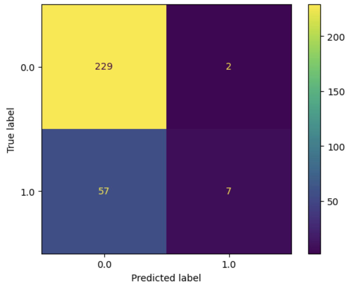

As you can see the model almost always predicts the majority class (0 - no kids). Because 79% of the data falls within this class, this is actually not a bad strategy. It leads to an accuracy of 79%!

Of course this is not what we want, we also want to model to make correct predictions for the minority class.

We thus have to deal with imbalanced data!

7. Dealing with imbalanced data

Challenge: How do deal with unbalanced data?

What do you think is a good way to deal with the unbalance in the target variable?

Show me the solution

There are multiple ways to deal with this:

Find a model that can handle unbalanced data better
Upsample the data (duplicate a proportion of the minority class samples)
Downsample the data (take a subset of the majority class samples)

Challenge: Balance the dataset

Go ahead and balance the training dataset using the upsampling strategy. Hint: Try googling first, but you can have a look at: https://vitalflux.com/handling-class-imbalance-sklearn-resample-python/

Show me the solution

PYTHON

from sklearn.utils import resample
#
# Create oversampled training data set for minority class
#
X_oversampled, y_oversampled = resample(X_train[y_train == 1],
                                        y_train[y_train == 1],
                                        replace=True,
                                        n_samples=X_train[y_train == 0].shape[0],
                                        random_state=123)
#
# Append the oversampled minority class to training data and related labels
#
X_balanced = pd.concat((X_train[y_train == 0], X_oversampled))
y_balanced = pd.concat((y_train[y_train == 0], y_oversampled))

Check that the data is indeed balanced:

PYTHON

y_balanced.mean()

0.5

Check that there is now indeed more data in the training set:

PYTHON

X_balanced.shape

OUTPUT

(1080, 4)

8. Train and evaluate the model trained on a balanced dataset

Now that we have balanced our dataset, we can see whether this improves the performance of our model!

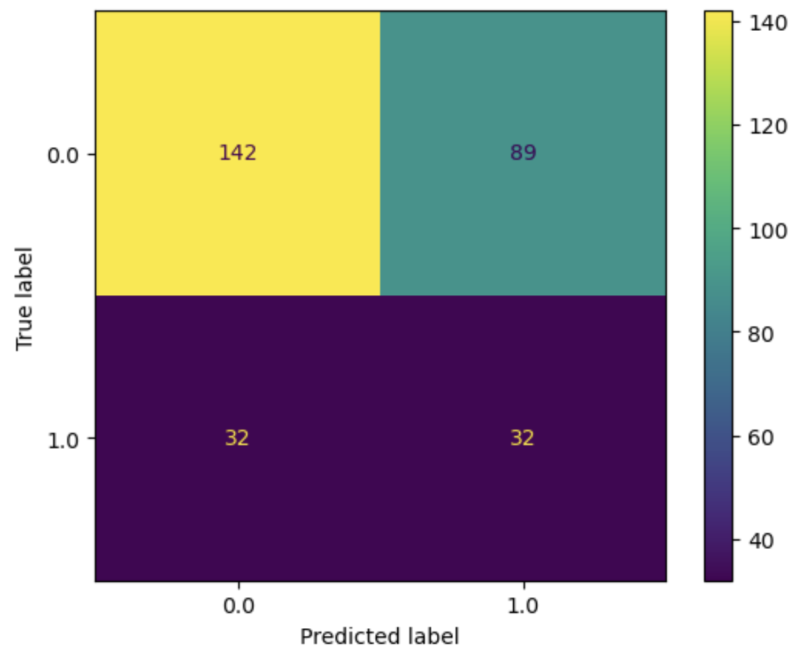
Challenge: Train the model on the balanced dataset

Train the model on the balanced dataset
Evaluate the model by visualizing the results. What do you see?

Show me the solution

PYTHON

_ = model.fit(X_balanced, y_balanced)
_ = ConfusionMatrixDisplay.from_estimator(model, X_test, y_test)

This already looks much better! The predictions are more balanced over the two classes, and are also quite often correct. So balancing the data helped a lot!

9. Use evaluation metrics to evaluate the model

So far we have used a confusion matrix to visually evaluate the model. When proceeding it would be better to use evaluation metrics for this.

Challenge: Evaluation metrics

Evaluate the model using the appropriate evaluation metrics. Hint: the dataset is unbalanced.

Show me the solution

Good evaluation metrics would be precision, recall, and F1-score for the positive class (getting a child in the next 3 years) This of course also makes sense, sense these are the metrics that are used in the benchmark.

Precision gives us a measure for how many of the households labeled as ‘fertile’ was that a correct prediction. Recall gives us a measure for how many of the households that are actually ‘fertile’ how many we correctly ‘detect’ as being fertile.

F1-score is the harmonic mean of the two.

PYTHON

from sklearn.metrics import precision_recall_fscore_support

y_pred = model.predict(X_test)
p, r, f, _ = precision_recall_fscore_support(y_test, y_pred, average='binary')
print(f'Precision: {p}, recall: {r}, F1-score: {f}')

Precision: 0.2644628099173554, recall: 0.5, F1-score: 0.34594594594594597

Challenge: Test your understanding of precision and recall by computing the scores by hand! You can use the numbers shown in the confusion matrix for this.

10. Adapt, train, evaluate. Adapt, train, evaluate.

Good job! You have now set up a simple, yet effective machine learning pipeline on a real-world problem. Notice that you already went through the machine learning cycle twice. From this point onward it is a matter of adapting your approach, train the model, evaluate the results. Again, and again, and again.

Of course there is still a lot of room for improvement. Every time you evaluate the results, try to come up with a shortlist of things that seem most promising to try out in the next cycle.

Challenge: Improving the model further

What ideas do you have to improve the model further?

Show me the solution

There is no right or wrong, but here are some pointers:

Include more features. You can think of automated feature selection to select features or go through the codebook by hand and select the most promising.
Engineer more features. You could try and create new features yourself, based on the variables in the dataset, or maybe combine a different dataset.
Try out different models.
Come up with a good baseline, to get a feeling for how good the model is performing.
Use hyperparameter tuning to find the best hyperparameters for a model.
Try out different preprocessing approaches
Deal with missing data differently. Try out imputation.