Registration and Segmentation with SITK

Overview

Questions

• What are SITK Images?
• How can registration be implemented in SITK?
• How can I segment an image in SITK?

Objectives

• Explain how to perform basic operations on SITK Images
• Explain when registration can be needed and how to register images with SITK
• Become familiar with basic segmentation algorithms available in SITK

Introduction

---

In the realm of medical imaging analysis, registration and segmentation play crucial roles. Registration aligns images, enabling the fusion of data or the tracking of changes over time. Segmentation identifies and labels objects of interest within images. Automation is essential due to high clinical demand, driving the development of robust algorithms for both processes. Moreover, many advanced segmentation techniques utilize image registration, whether implicitly or explicitly.

SimpleITK (SITK) is a simplified programming interface to the algorithms and data structures of the Insight Toolkit (ITK) for segmentation, registration and advanced image analysis, available in many programming languages (e.g., C++, Python, R, Java, C#, Lua, Ruby).

SITK is part of the Insight Software Consortium a non-profit educational consortium dedicated to promoting and maintaining open-source, freely available software for medical image analysis. Its copyright is held by NumFOCUS, and the software is distributed under the Apache License 2.0.

In this episode, we use a hands-on approach utilizing Python to show how to use SITK for performing registration and segmentation tasks in medical imaging use cases.

Fundamental Concepts

---

In this section, we’ll cover some fundamental image processing operations using SITK, such as reading and writing images, accessing pixel values, and resampling images.

Images

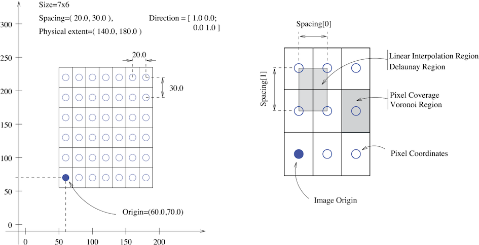
The fundamental tenet of an image in ITK and consequentially in SITK is that an image is defined by a set of points on a grid occupying a physical region in space . This significantly differs from many other image analysis libraries that treat an image as an array which has two implications: (1) pixel/voxel spacing is assumed to be isotropic and (2) there is no notion of an image’s location in physical space.

SITK images are multi-dimensional (the default configuration includes images from two dimensional up to five dimensional) and can be a scalar, labelmap (scalar with run length encoding), complex value or have an arbitrary number of scalar channels (also known as a vector image). The region in physical space which an image occupies is defined by the image’s:

1. Origin (vector like type) - location in the world coordinate system of the voxel with all zero indexes.
2. Spacing (vector like type) - distance between pixels along each of the dimensions.
3. Size (vector like type) - number of pixels in each dimension.
4. Direction cosine matrix (vector like type representing matrix in row major order) - direction of each of the axes corresponding to the matrix columns.

The following figure illustrates these concepts.

An image in SITK occupies a region in physical space which is defined by its meta-data (origin, size, spacing, and direction cosine matrix). Note that the image’s physical extent starts half a voxel before the origin and ends half a voxel beyond the last voxel.

In SITK, when we construct an image we specify its dimensionality, size and pixel type, all other components are set to reasonable default values:

1. Origin - all zeros.
2. Spacing - all ones.
3. Direction - identity.
4. Intensities in all channels - all zero.

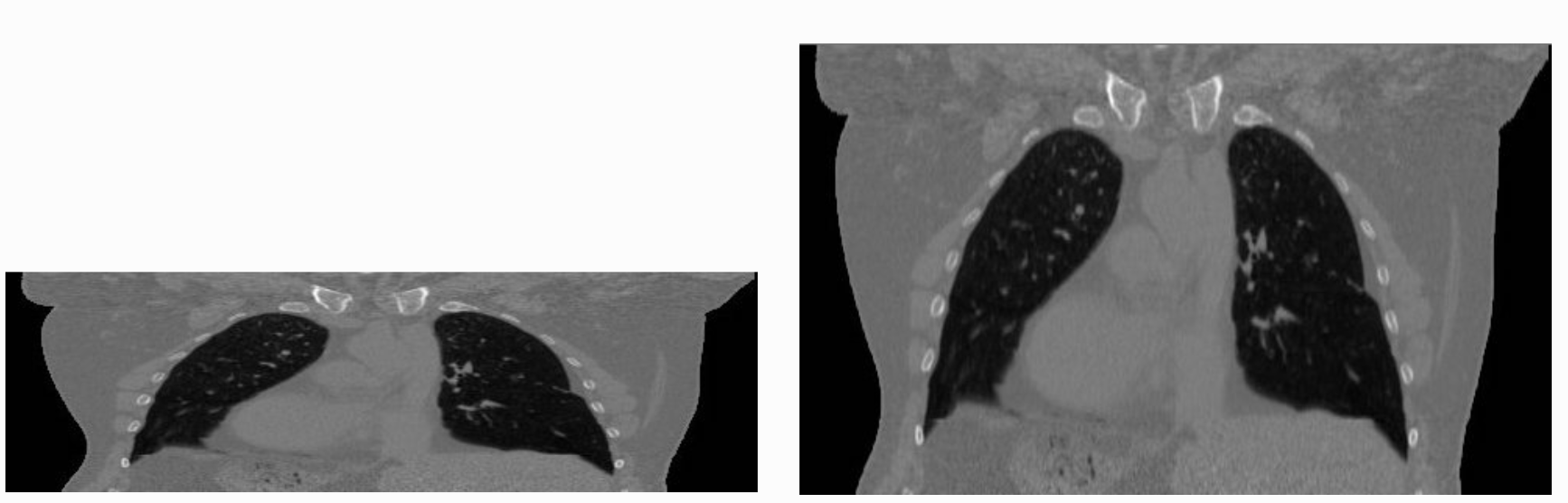
The tenet that images occupy a spatial location in the physical world has to do with the original application domain of ITK and SITK, medical imaging. In that domain images represent anatomical structures with metric sizes and spatial locations. Additionally, the spacing between voxels is often non-isotropic (most commonly the spacing along the inferior-superior/foot-to-head direction is larger). Viewers that treat images as an array will display a distorted image as shown below:

The same image displayed with a viewer that is not aware of spatial meta-data (left image) and one that is aware (right image). The image’s pixel spacing is (0.97656, 2.0)mm.

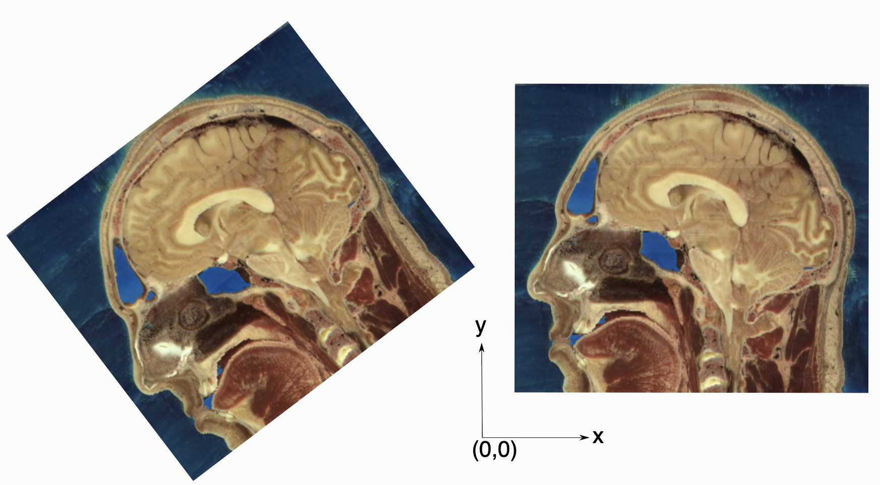
As an image is also defined by its spatial location, two images with the same pixel data and spacing may not be considered equivalent. Think of two CT scans of the same patient acquired at different sites. The following figure illustrates the notion of spatial location in the physical world, the two images are considered different even though the intensity values and pixel spacing are the same.

Two images with exactly the same pixel data, positioned in the world coordinate system. In SITK these are not considered the same image, because they occupy different spatial locations.

As SITK images occupy a physical region in space, the quantities defining this region have metric units (cm, mm, etc.). In general SITK assumes units are in millimeters (historical reasons, due to DICOM standard). In practice SITK is not aware of the specific units associated with each image, it just assumes that they are consistent. Thus, it is up to you the developer to ensure that all of the images you read and created are using the same units.

A SITK image can have an arbitrary number of channels with the content of the channels being a scalar or complex value. This is determined when an image is created.

In the medical domain, many image types have a single scalar channel (e.g. CT, US). Another common image type is a three channel image where each channel has scalar values in [0,255], often people refer to such an image as an RGB image. This terminology implies that the three channels should be interpreted using the RGB color space. In some cases you can have the same image type, but the channel values represent another color space, such as HSV (it decouples the color and intensity information and is a bit more invariant to illumination changes). SITK has no concept of color space, thus in both cases it will simply view a pixel value as a 3-tuple.

Let’s read an example of human brain CT, and let’s explore it with SITK.

PYTHON

%matplotlib inline
import matplotlib.pyplot as plt
import SimpleITK as sitk

img_volume = sitk.ReadImage("data/sitk/A1_grayT1.nrrd")

print(type(img_volume))
print(img_volume.GetOrigin())
print(img_volume.GetSpacing())
print(img_volume.GetDirection())

OUTPUT

<class 'SimpleITK.SimpleITK.Image'>
(-77.625, -107.625, 119.625)
(0.75, 0.75, 0.75)
(0.0, 0.0, 1.0, 1.0, 0.0, 0.0, 0.0, -1.0, 0.0)

The function sitk.ReadImage loads the file as a SimpleITK.SimpleITK.Image instance, and then we can access useful methods to get an idea of how the image/s contained in the file is/are. The size of the image’s dimensions have explicit accessors:

PYTHON

print(img_volume.GetSize())
print(img_volume.GetWidth())
print(img_volume.GetHeight())
print(img_volume.GetDepth())
print(img_volume.GetNumberOfComponentsPerPixel())
print(img_volume.GetPixelIDTypeAsString())

OUTPUT

(288, 320, 208)
288
320
208
1
32-bit float

Just inspecting these accessors, we deduce that the file contains a volume made of 208 images, each made of 288x320 pixels and one channel only (grayscale).

SITK Conventions

• Image access is in x,y,z order, image.GetPixel(x,y,z) or image[x,y,z], with zero based indexing.
• If the output of an ITK filter has non-zero starting index, then the index will be set to 0, and the origin adjusted accordingly.

Displaying Images

While SITK does not do visualization, it does contain a built in Show method. This function writes the image out to disk and than launches a program for visualization. By default it is configured to use ImageJ, because it is readily supports all the image types which SITK has and load very quickly.

PYTHON

sitk.Show?

SITK provides two options for invoking an external viewer, use a procedural interface (the Show function) or an object oriented one. For more details about them, please refer to this notebook from the official documentation.

In this episode we will convert SITK images to numpy arrays, and we will plot them as such.

Images as Arrays

We have two options for converting from SITK to a numpy array:

• GetArrayFromImage(): returns a copy of the image data. You can then freely modify the data as it has no effect on the original SITK image.
• GetArrayViewFromImage(): returns a view on the image data which is useful for display in a memory efficient manner. You cannot modify the data and the view will be invalid if the original SITK image is deleted.

The order of index and dimensions need careful attention during conversion. ITK’s Image class has a GetPixel which takes an ITK Index object as an argument, which is ordered as (x,y,z). This is the convention that SITK’s Image class uses for the GetPixel method and slicing operator as well. In numpy, an array is indexed in the opposite order (z,y,x). Also note that the access to channels is different. In SITK you do not access the channel directly, rather the pixel value representing all channels for the specific pixel is returned and you then access the channel for that pixel. In the numpy array you are accessing the channel directly. Let’s see this in an example:

PYTHON

import numpy as np

multi_channel_3Dimage = sitk.Image([2, 4, 8], sitk.sitkVectorFloat32, 5)
x = multi_channel_3Dimage.GetWidth() - 1
y = multi_channel_3Dimage.GetHeight() - 1
z = multi_channel_3Dimage.GetDepth() - 1
multi_channel_3Dimage[x, y, z] = np.random.random(
    multi_channel_3Dimage.GetNumberOfComponentsPerPixel()
)

nda = sitk.GetArrayFromImage(multi_channel_3Dimage)

print("Image size: " + str(multi_channel_3Dimage.GetSize()))
print("Numpy array size: " + str(nda.shape))

# Notice the index order and channel access are different:
print("First channel value in image: " + str(multi_channel_3Dimage[x, y, z][0]))
print("First channel value in numpy array: " + str(nda[z, y, x, 0]))

OUTPUT

Image size: (2, 4, 8)
Numpy array size: (8, 4, 2, 5)
First channel value in image: 0.5384010076522827
First channel value in numpy array: 0.538401

Going back to the loaded file, let’s plot the array version of the volume slice from the middle of the stack, along the z axis, using different color maps:

PYTHON

npa = sitk.GetArrayViewFromImage(img_volume)

# Display the image slice from the middle of the stack, z axis
z = int(img_volume.GetDepth() / 2)
npa_zslice = sitk.GetArrayViewFromImage(img_volume)[z, :, :]

# Three plots displaying the same data, how do we deal with the high dynamic range?
fig = plt.figure(figsize=(10, 3))

fig.add_subplot(1, 3, 1)
plt.imshow(npa_zslice)
plt.title("default colormap", fontsize=10)
plt.axis("off")

fig.add_subplot(1, 3, 2)
plt.imshow(npa_zslice, cmap=plt.cm.Greys_r)
plt.title("grey colormap", fontsize=10)
plt.axis("off")

fig.add_subplot(1, 3, 3)
plt.title(
    "grey colormap,\n scaling based on volumetric min and max values", fontsize=10
)
plt.imshow(npa_zslice, cmap=plt.cm.Greys_r, vmin=npa.min(), vmax=npa.max())
plt.axis("off")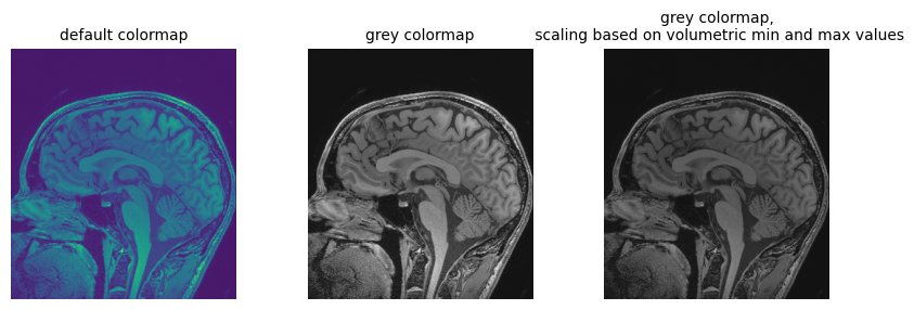

We can also do the reverse, i.e. converting a numpy array to the SITK Image:

PYTHON

img_zslice = sitk.GetImageFromArray(npa_zslice)
print(type(img_zslice))

OUTPUT

<class 'SimpleITK.SimpleITK.Image'>

We can also plot multiple slices at the same time, for better inspecting the volume:

PYTHON

img_xslices = [img_volume[x,:,:] for x in range(50, 200, 30)]
img_yslices = [img_volume[:,y,:] for y in range(50, 200, 30)]
img_zslices = [img_volume[:,:,z] for z in range(50, 200, 30)]

tile_x = sitk.Tile(img_xslices, [1,0])
tile_y = sitk.Tile(img_yslices, [1,0])
tile_z = sitk.Tile(img_zslices, [1,0])

nda_xslices = sitk.GetArrayViewFromImage(tile_x)
nda_yslices = sitk.GetArrayViewFromImage(tile_y)
nda_zslices = sitk.GetArrayViewFromImage(tile_z)

fig, (ax1, ax2, ax3) = plt.subplots(1,3)
ax1.imshow(nda_xslices, cmap=plt.cm.Greys_r)
ax2.imshow(nda_yslices, cmap=plt.cm.Greys_r)
ax3.imshow(nda_zslices, cmap=plt.cm.Greys_r)
ax1.set_title('X slices')
ax2.set_title('Y slices')
ax3.set_title('Z slices')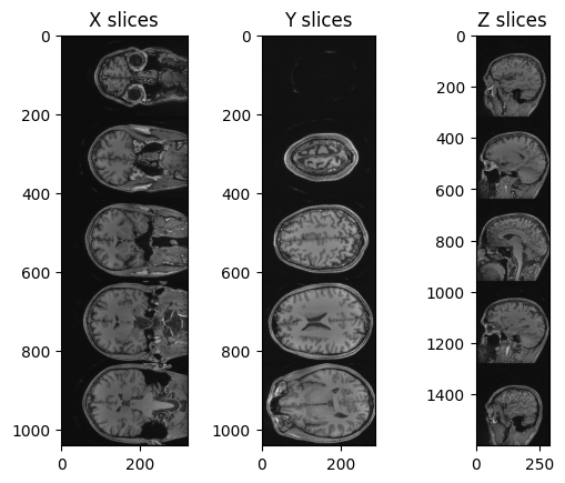

Operations like slice indexing, cropping, flipping, … can be performed on SITK images very similarly as it is usually done in numpy. Note that slicing of SITK images returns a copy of the image data, similarly to slicing Python lists, and differently from the “view” returned by slicing numpy arrays.

PYTHON

n_slice = 150

# Original slice
plt.imshow(sitk.GetArrayViewFromImage(img_volume[:, :, n_slice]), cmap="gray")

PYTHON

# Cropping
plt.imshow(sitk.GetArrayViewFromImage(img_volume[:, :100, n_slice]), cmap="gray")

PYTHON

# Flipping
plt.imshow(sitk.GetArrayViewFromImage(img_volume[:, ::-1, n_slice]), cmap="gray")

PYTHON

# Subsampling
plt.imshow(sitk.GetArrayViewFromImage(img_volume[:, ::3, n_slice]), cmap="gray")

PYTHON

# Comparative operators
plt.imshow(sitk.GetArrayViewFromImage(img_volume[:, :, n_slice] > 90), cmap="gray")

PYTHON

# Draw a square
draw_square = sitk.GetArrayFromImage(img_volume[:, :, n_slice])
draw_square[0:100,0:100] = draw_square.max()
plt.imshow(draw_square, cmap="gray")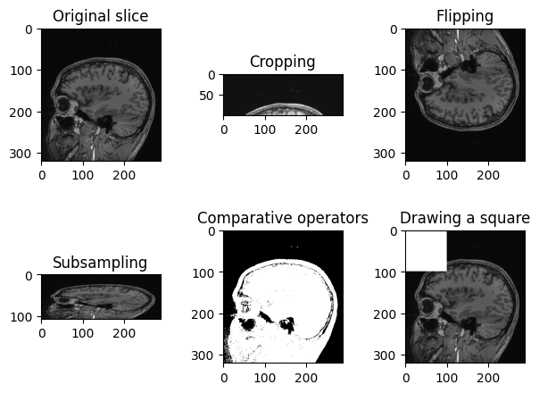

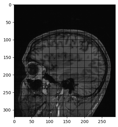
Another example of operation we can perform is creating a grid mask and apply it to an image:

PYTHON

img_zslice = img_volume[:, :, n_slice]
# Create a grid and use as mask
grid_image = sitk.GridSource(
    outputPixelType=sitk.sitkUInt16,
    size=img_zslice.GetSize(),
    sigma=(0.1, 0.1),
    gridSpacing=(20.0, 20.0),
)

# zero out the values in the original image that correspond to
# the grid lines in the grid_image
img_zslice[grid_image == 0] = 0
nda = sitk.GetArrayViewFromImage(slice)
plt.imshow(nda, cmap="gray")

Challenge: Fix the Error (Optional)

By running the lines of code above for masking the slice with the grid, you will get an error. Can you guess what is it about?

Show me the solution

By default, SITK creates images centered in the origin, which all ones spacing. We need to have the same values in the grid and in the image in order to superimpose the first to the latter.

PYTHON

grid_image.SetOrigin(img_zslice.GetOrigin())
grid_image.SetSpacing(img_zslice.GetSpacing())

Add these two lines to the code above, after the creation of the grid. Everything should work fine now. Remember that making such changes to an image already containing data should be done cautiously.

Meta-dictionaries

SITK can read (and write) images stored in a single file, or a set of files (e.g. DICOM series).

Images stored in the DICOM format have a meta-data dictionary associated with them, which is populated with the DICOM tags. When a DICOM series is read as a single image, the meta-data information is not available since DICOM tags are specific to each file. If you need the meta-data, you have three options:

1. Using the object oriented interface’s ImageSeriesReader class, configure it to load the tags using the MetaDataDictionaryArrayUpdateOn method and possibly the LoadPrivateTagsOn method if you need the private tags. Once the series is read you can access the meta-data from the series reader using the GetMetaDataKeys, HasMetaDataKey, and GetMetaData.

2. Using the object oriented interface’s ImageFileReader, set a specific slice’s file name and only read it’s meta-data using the ReadImageInformation method which only reads the meta-data but not the bulk pixel information. Once the meta-data is read you can access it from the file reader using the GetMetaDataKeys, HasMetaDataKey, and GetMetaData.

3. Using the object oriented interface’s ImageFileReader, set a specific slice’s file name and read it. Or using the procedural interface’s, ReadImage function, read a specific file. You can then access the meta-data directly from the Image using the GetMetaDataKeys, HasMetaDataKey, and GetMetaData.

Note: When reading an image series, via the ImageSeriesReader or via the procedural ReadImage interface, the images in the list are assumed to be ordered correctly (GetGDCMSeriesFileNames ensures this for DICOM). If the order is incorrect, the image will be read, but its spacing and possibly the direction cosine matrix will be incorrect.

Let’s read in a digital x-ray image saved in a DICOM file format, and let’s print the metadata’s keys:

PYTHON

img_xray = sitk.ReadImage('data/sitk/digital_xray.dcm')

for key in img_xray.GetMetaDataKeys():
    print(f'"{key}":"{img_xray.GetMetaData(key)}"')

OUTPUT

"0008|0005":"ISO_IR 100"
"0008|0012":"20180713"
"0008|0013":"233245.431"
"0008|0016":"1.2.840.10008.5.1.4.1.1.7"
"0008|0018":"2.25.225981116244996633889747723103230447077"
"0008|0020":"20160208"
"0008|0060":"XC"
"0020|000d":"2.25.59412532821774470466514450673479191872"
"0020|000e":"2.25.149748537243964334146339164752570719260"
"0028|0002":"3"
"0028|0004":"YBR_FULL_422"
"0028|0006":"0"
"0028|0010":"357"
"0028|0011":"371"
"0028|0100":"8"
"0028|0101":"8"
"0028|0102":"7"
"0028|0103":"0"
"ITK_original_direction":"[UNKNOWN_PRINT_CHARACTERISTICS]
"
"ITK_original_spacing":"[UNKNOWN_PRINT_CHARACTERISTICS]
"

Reading a DICOM:

• Many libraries allow you to read DICOM metadata.
• PyDICOM will be explored for this task later.
• If you are already using SITK, you will usually not need an extra library to get DICOM metadata.
• Many libraries have some basic DICOM functionality, check the documentation before adding extra dependencies.

Generally speaking, SITK represents color images as multi-channel images independent of a color space. It is up to you to interpret the channels correctly based on additional color space knowledge prior to using them for display or any other purpose.

Things to note: 1. When using SITK to read a color DICOM image, the channel values will be transformed to the RGB color space. 2. When using SITK to read a scalar image, it is assumed that the lowest intensity value is black and highest white. If the photometric interpretation tag is MONOCHROME2 (lowest value displayed as black) nothing is done. If it is MONOCHROME1 (lowest value displayed as white), the pixel values are inverted.

PYTHON

print(f'Image Modality: {img_xray.GetMetaData("0008|0060")}')
print(img_xray.GetNumberOfComponentsPerPixel())

OUTPUT

Image Modality: XC
3

“0008|0060” is a code indicating the modality, and “XC” stays for “External-camera Photography”.

Grayscale Images Stored as sRGB

“digital_xray.dcm” image is sRGB, even if an x-ray should be a single channel gray scale image. In some cases looks may be deceiving. Gray scale images are not always stored as a single channel image. In some cases an image that looks like a gray scale image is actually a three channel image with the intensity values repeated in each of the channels. Even worse, some gray scale images can be four channel images with the channels representing RGBA and the alpha channel set to all 255. This can result in a significant waste of memory and computation time. Always become familiar with your data.

We can convert sRGB to gray scale:

PYTHON

nda_xray = sitk.GetArrayViewFromImage(img_xray)
plt.imshow(np.squeeze(nda_xray))

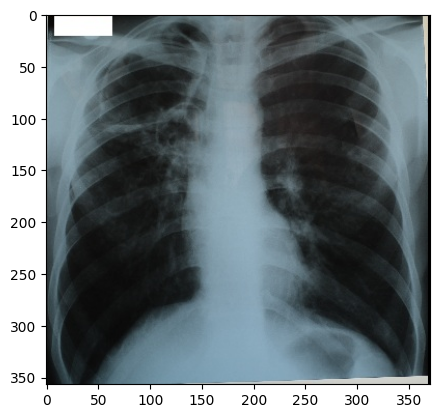
PYTHON

def srgb2gray(image):
    # Convert sRGB image to gray scale and rescale results to [0,255]
    channels = [
        sitk.VectorIndexSelectionCast(image, i, sitk.sitkFloat32)
        for i in range(image.GetNumberOfComponentsPerPixel())
    ]
    # linear mapping
    I = 1 / 255.0 * (0.2126 * channels[0] + 0.7152 * channels[1] + 0.0722 * channels[2])
    # nonlinear gamma correction
    I = (
        I * sitk.Cast(I <= 0.0031308, sitk.sitkFloat32) * 12.92
        + I ** (1 / 2.4) * sitk.Cast(I > 0.0031308, sitk.sitkFloat32) * 1.055
        - 0.055
    )
    return sitk.Cast(sitk.RescaleIntensity(I), sitk.sitkUInt8)

img_xray_gray = srgb2gray(img_xray)
nda = sitk.GetArrayViewFromImage(img_xray_gray)
plt.imshow(np.squeeze(nda), cmap="gray")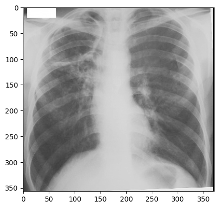

Transforms

SITK supports two types of spatial transforms, ones with a global (unbounded) spatial domain and ones with a bounded spatial domain. Points in SITK are mapped by the transform using the TransformPoint method.

All global domain transforms are of the form:

\(T(x) = A(x - c) + t + c\)

The nomenclature used in the documentation refers to the components of the transformations as follows:

• Matrix - the matrix \(A\).
• Center - the point \(c\).
• Translation - the vector \(t\).
• Offset - the expression \(t + c - Ac\).

A variety of global 2D and 3D transformations are available (translation, rotation, rigid, similarity, affine…). Some of these transformations are available with various parameterizations which are useful for registration purposes.

The second type of spatial transformation, bounded domain transformations, are defined to be identity outside their domain. These include the B-spline deformable transformation, often referred to as Free-Form Deformation, and the displacement field transformation.

The B-spline transform uses a grid of control points to represent a spline based transformation. To specify the transformation the user defines the number of control points and the spatial region which they overlap. The spline order can also be set, though the default of cubic is appropriate in most cases. The displacement field transformation uses a dense set of vectors representing displacement in a bounded spatial domain. It has no implicit constraints on transformation continuity or smoothness.

Finally, SITK supports a composite transformation with either a bounded or global domain. This transformation represents multiple transformations applied one after the other \(T_0(T_1(T_2(...T_n(p))))\). The semantics are stack based, that is, first in last applied:

PYTHON

composite_transform = CompositeTransform([T0, T1])
composite_transform.AddTransform(T2)

For more details about SITK transformation types and examples, see this tutorial notebook.

Resampling

Resampling, as the verb implies, is the action of sampling an image, which itself is a sampling of an original continuous signal.

Generally speaking, resampling in SITK involves four components:

1. Image - the image we resample, given in coordinate system \(m\).
2. Resampling grid - a regular grid of points given in coordinate system \(f\) which will be mapped to coordinate system \(m\).
3. Transformation \(T_f^m\) - maps points from coordinate system \(f\) to coordinate system \(m\), \(^mp=T_f^m(^fp)\).
4. Interpolator - method for obtaining the intensity values at arbitrary points in coordinate system \(m\) from the values of the points defined by the Image.

While SITK provides a large number of interpolation methods, the two most commonly used are sitkLinear and sitkNearestNeighbor. The former is used for most interpolation tasks and is a compromise between accuracy and computational efficiency. The later is used to interpolate labeled images representing a segmentation. It is the only interpolation approach which will not introduce new labels into the result.

The SITK interface includes three variants for specifying the resampling grid:

1. Use the same grid as defined by the resampled image.
2. Provide a second, reference, image which defines the grid.
3. Specify the grid using: size, origin, spacing, and direction cosine matrix.

Points that are mapped outside of the resampled image’s spatial extent in physical space are set to a constant pixel value which you provide (default is zero).

It is not uncommon to end up with an empty (all black) image after resampling. This is due to:

1. Using wrong settings for the resampling grid (not too common, but does happen).
2. Using the inverse of the transformation \(T_f^m\). This is a relatively common error, which is readily addressed by invoking the transformation’s GetInverse method.

Let’s try to plot multiple slices across different axis for the image “training_001_mr_T1.mha”.

PYTHON

img_volume = sitk.ReadImage("data/sitk/training_001_mr_T1.mha")
print(img_volume.GetSize())
print(img_volume.GetSpacing())

OUTPUT

(256, 256, 26)
(1.25, 1.25, 4.0)

We can plot the slices as we did before:

PYTHON

img_xslices = [img_volume[x,:,:] for x in range(50, 200, 30)]
img_yslices = [img_volume[:,y,:] for y in range(50, 200, 30)]
img_zslices = [img_volume[:,:,z] for z in range(1, 25, 3)]

tile_x = sitk.Tile(img_xslices, [1,0])
tile_y = sitk.Tile(img_yslices, [1,0])
tile_z = sitk.Tile(img_zslices, [1,0])

nda_xslices = sitk.GetArrayViewFromImage(tile_x)
nda_yslices = sitk.GetArrayViewFromImage(tile_y)
nda_zslices = sitk.GetArrayViewFromImage(tile_z)

fig, (ax1, ax2, ax3) = plt.subplots(1,3)
ax1.imshow(nda_xslices, cmap=plt.cm.Greys_r)
ax2.imshow(nda_yslices, cmap=plt.cm.Greys_r)
ax3.imshow(nda_zslices, cmap=plt.cm.Greys_r)
ax1.set_title('X slices')
ax2.set_title('Y slices')
ax3.set_title('Z slices')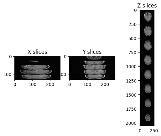

Challenge: Distorted Images

What is the main difference with the first image we plotted (“A1_grayT1.nrrd”)?

Show me the solution

In this case, there are only 26 images in the volume and the spacing between voxels is non-isotropic, and in particular it is the same across x- and y-axis, but it differs across the z-axis.

We can fix the distortion by resampling the volume along the z-axis, which has a different spacing (i.e., 4mm), and make it match with the other two spacing measures (i.e., 1.25mm):

PYTHON

def resample_img(image, out_spacing=[1.25, 1.25, 1.25]):
    
    # Resample images to 1.25mm spacing
    original_spacing = image.GetSpacing()
    original_size = image.GetSize()

    out_size = [
        int(np.round(original_size[0] * (original_spacing[0] / out_spacing[0]))),
        int(np.round(original_size[1] * (original_spacing[1] / out_spacing[1]))),
        int(np.round(original_size[2] * (original_spacing[2] / out_spacing[2])))]

    resample = sitk.ResampleImageFilter()
    resample.SetOutputSpacing(out_spacing)
    resample.SetSize(out_size)
    resample.SetOutputDirection(image.GetDirection())
    resample.SetOutputOrigin(image.GetOrigin())
    resample.SetTransform(sitk.Transform())
    resample.SetDefaultPixelValue(image.GetPixelIDValue())
    resample.SetInterpolator(sitk.sitkBSpline)

    return resample.Execute(image)

resampled_sitk_img = resample_img(img_volume)

print(resampled_sitk_img.GetSize())
print(resampled_sitk_img.GetSpacing())

OUTPUT

(256, 256, 83)
(1.25, 1.25, 1.25)

Registration

---

Image registration involves spatially transforming the source/moving image(s) to align with the target image. More specifically, the goal of registration is to estimate the transformation which maps points from one image to the corresponding points in another image. The transformation estimated via registration is said to map points from the fixed image (target image) coordinate system to the moving image (source image) coordinate system.

Many Ways to Do Registration:

• Several libraries offer built-in registration functionalities.
• Registration can be performed with DIPY (mentioned in the MRI episode), specifically for diffusion imaging using the SymmetricDiffeomorphicRegistration functionality.
• NiBabel includes a function in its processing module that allows resampling or conforming one NIfTI image into the space of another.
• SITK provides robust registration capabilities and allows you to code your own registration algorithms.
• To maintain cleaner and more efficient code, it’s advisable to use as few libraries as possible and avoid those that may create conflicts.

SITK provides a configurable multi-resolution registration framework, implemented in the ImageRegistrationMethod class. In addition, a number of variations of the Demons registration algorithm are implemented independently from this class as they do not fit into the framework.

The task of registration is formulated using non-linear optimization which requires an initial estimate. The two most common initialization approaches are (1) Use the identity transform (a.k.a. forgot to initialize). (2) Align the physical centers of the two images (see CenteredTransformInitializerFilter). If after initialization there is no overlap between the images, registration will fail. The closer the initialization transformation is to the actual transformation, the higher the probability of convergence to the correct solution.

If your registration involves the use of a global domain transform (described here), you should also set an appropriate center of rotation. In many cases you want the center of rotation to be the physical center of the fixed image (the CenteredTransformCenteredTransformInitializerFilter ensures this). This is of significant importance for registration convergence due to the non-linear nature of rotation. When the center of rotation is far from our physical region of interest (ROI), a small rotational angle results in a large displacement. Think of moving the pivot/fulcrum point of a lever. For the same rotation angle, the farther you are from the fulcrum the larger the displacement. For numerical stability we do not want our computations to be sensitive to very small variations in the rotation angle, thus the ideal center of rotation is the point which minimizes the distance to the farthest point in our ROI:

\(p_{center} = arg_{p_{rotation}} min dist (p_{rotation}, \{p_{roi}\})\)

Without additional knowledge we can only assume that the ROI is the whole fixed image. If your ROI is only in a sub region of the image, a more appropriate point would be the center of the oriented bounding box of that ROI.

To create a specific registration instance using the ImageRegistrationMethod you need to select several components which together define the registration instance:

1. Transformation
   • It defines the mapping between the two images.
2. Similarity metric
   • It reflects the relationship between the intensities of the images (identity, affine, stochastic…).
3. Optimizer.
   • When selecting the optimizer you will also need to configure it (e.g. set the number of iterations).
4. Interpolator.
   • In most cases linear interpolation, the default setting, is sufficient.

Let’s see now an example where we want to use registration for aligning two volumes relative to the same patient, one being a CT scan and the second being a MRI sequence T1-weighted scan. We first read the images, casting the pixel type to that required for registration (Float32 or Float64) and look at them:

PYTHON

from ipywidgets import interact, fixed
from IPython.display import clear_output
import os

OUTPUT_DIR = "data/sitk/"
fixed_image =  sitk.ReadImage(f"{OUTPUT_DIR}training_001_ct.mha", sitk.sitkFloat32)
moving_image = sitk.ReadImage(f"{OUTPUT_DIR}training_001_mr_T1.mha", sitk.sitkFloat32)

print(f"Origin for fixed image: {fixed_image.GetOrigin()}, moving image: {moving_image.GetOrigin()}")
print(f"Spacing for fixed image: {fixed_image.GetSpacing()}, moving image: {moving_image.GetSpacing()}")
print(f"Size for fixed image: {fixed_image.GetSize()}, moving image: {moving_image.GetSize()}")
print(f"Number Of Components Per Pixel for fixed image: {fixed_image.GetNumberOfComponentsPerPixel()}, moving image: {moving_image.GetNumberOfComponentsPerPixel()}")

# Callback invoked by the interact IPython method for scrolling through the image stacks of
# the two images (moving and fixed).
def display_images(fixed_image_z, moving_image_z, fixed_npa, moving_npa):
    # Create a figure with two subplots and the specified size.
    plt.subplots(1,2,figsize=(10,8))
    
    # Draw the fixed image in the first subplot.
    plt.subplot(1,2,1)
    plt.imshow(fixed_npa[fixed_image_z,:,:],cmap=plt.cm.Greys_r)
    plt.title('fixed/target image')
    plt.axis('off')
    
    # Draw the moving image in the second subplot.
    plt.subplot(1,2,2)
    plt.imshow(moving_npa[moving_image_z,:,:],cmap=plt.cm.Greys_r)
    plt.title('moving/source image')
    plt.axis('off')
    
    plt.show()

interact(
    display_images,
    fixed_image_z = (0,fixed_image.GetSize()[2]-1),
    moving_image_z = (0,moving_image.GetSize()[2]-1),
    fixed_npa = fixed(sitk.GetArrayViewFromImage(fixed_image)),
    moving_npa = fixed(sitk.GetArrayViewFromImage(moving_image)))

OUTPUT

Origin for fixed image: (0.0, 0.0, 0.0), moving image: (0.0, 0.0, 0.0)
Spacing for fixed image: (0.653595, 0.653595, 4.0), moving image: (1.25, 1.25, 4.0)
Size for fixed image: (512, 512, 29), moving image: (256, 256, 26)
Number Of Components Per Pixel for fixed image: 1, moving image: 1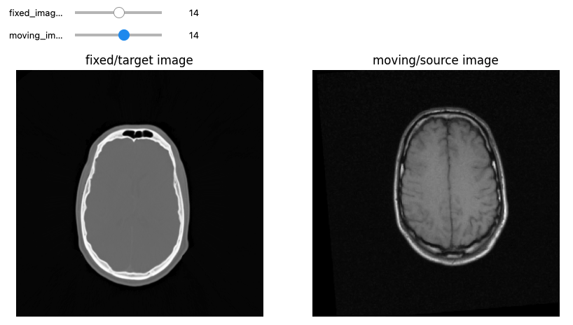

We can use the CenteredTransformInitializer to align the centers of the two volumes and set the center of rotation to the center of the fixed image:

PYTHON

# Callback invoked by the IPython interact method for scrolling and
# modifying the alpha blending of an image stack of two images that
# occupy the same physical space. 
def display_images_with_alpha(image_z, alpha, fixed, moving):
    img = (1.0 - alpha)*fixed[:,:,image_z] + alpha*moving[:,:,image_z] 
    plt.imshow(sitk.GetArrayViewFromImage(img),cmap=plt.cm.Greys_r)
    plt.axis('off')
    plt.show()

initial_transform = sitk.CenteredTransformInitializer(fixed_image, 
                                                      moving_image, 
                                                      sitk.Euler3DTransform(), 
                                                      sitk.CenteredTransformInitializerFilter.GEOMETRY)

moving_resampled = sitk.Resample(moving_image, fixed_image, initial_transform, sitk.sitkLinear, 0.0, moving_image.GetPixelID())

interact(
    display_images_with_alpha,
    image_z = (0,fixed_image.GetSize()[2]-1),
    alpha = (0.0,1.0,0.05),
    fixed = fixed(fixed_image),
    moving = fixed(moving_resampled))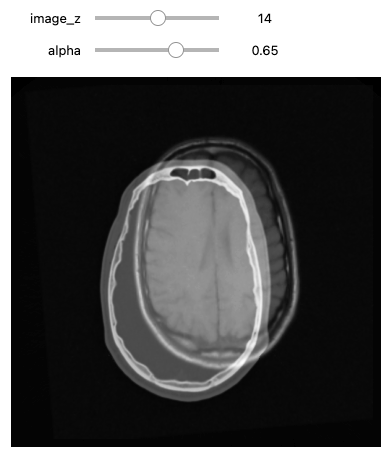

The specific registration task at hand estimates a 3D rigid transformation between images of different modalities. There are multiple components from each group (optimizers, similarity metrics, interpolators) that are appropriate for the task. Note that each component selection requires setting some parameter values. We have made the following choices:

• Similarity metric, mutual information (Mattes MI):
  • Number of histogram bins, 50.
  • Sampling strategy, random.
  • Sampling percentage, 1%.
• Interpolator, sitkLinear.
• Optimizer, gradient descent:
  • Learning rate, step size along traversal direction in parameter space, 1.0.
  • Number of iterations, maximal number of iterations, 100.
  • Convergence minimum value, value used for convergence checking in conjunction with the energy profile of the similarity metric that is estimated in the given window size, 1e-6.
  • Convergence window size, number of values of the similarity metric which are used to estimate the energy profile of the similarity metric, 10.

We perform registration using the settings given above, and by taking advantage of the built in multi-resolution framework, we use a three tier pyramid.

In this example we plot the similarity metric’s value during registration. Note that the change of scales in the multi-resolution framework is readily visible.

PYTHON

# Callback invoked when the StartEvent happens, sets up our new data.
def start_plot():
    global metric_values, multires_iterations
    
    metric_values = []
    multires_iterations = []

# Callback invoked when the EndEvent happens, do cleanup of data and figure.
def end_plot():
    global metric_values, multires_iterations
    
    del metric_values
    del multires_iterations
    # Close figure, we don't want to get a duplicate of the plot latter on.
    plt.close()

# Callback invoked when the sitkMultiResolutionIterationEvent happens, update the index into the 
# metric_values list. 
def update_multires_iterations():
    global metric_values, multires_iterations
    multires_iterations.append(len(metric_values))

# Callback invoked when the IterationEvent happens, update our data and display new figure.
def plot_values(registration_method):
    global metric_values, multires_iterations
    
    metric_values.append(registration_method.GetMetricValue())                                       
    # Clear the output area (wait=True, to reduce flickering), and plot current data
    clear_output(wait=True)
    # Plot the similarity metric values
    plt.plot(metric_values, 'r')
    plt.plot(multires_iterations, [metric_values[index] for index in multires_iterations], 'b*')
    plt.xlabel('Iteration Number',fontsize=12)
    plt.ylabel('Metric Value',fontsize=12)
    plt.show()


registration_method = sitk.ImageRegistrationMethod()

# Similarity metric settings.
registration_method.SetMetricAsMattesMutualInformation(numberOfHistogramBins=50)
registration_method.SetMetricSamplingStrategy(registration_method.RANDOM)
registration_method.SetMetricSamplingPercentage(0.01)

registration_method.SetInterpolator(sitk.sitkLinear)

# Optimizer settings.
registration_method.SetOptimizerAsGradientDescent(learningRate=1.0, numberOfIterations=100, convergenceMinimumValue=1e-6, convergenceWindowSize=10)
registration_method.SetOptimizerScalesFromPhysicalShift()

# Setup for the multi-resolution framework.            
registration_method.SetShrinkFactorsPerLevel(shrinkFactors = [4,2,1])
registration_method.SetSmoothingSigmasPerLevel(smoothingSigmas=[2,1,0])
registration_method.SmoothingSigmasAreSpecifiedInPhysicalUnitsOn()

# Don't optimize in-place, we would possibly like to run this cell multiple times.
registration_method.SetInitialTransform(initial_transform, inPlace=False)

# Connect all of the observers so that we can perform plotting during registration.
registration_method.AddCommand(sitk.sitkStartEvent, start_plot)
registration_method.AddCommand(sitk.sitkEndEvent, end_plot)
registration_method.AddCommand(sitk.sitkMultiResolutionIterationEvent, update_multires_iterations) 
registration_method.AddCommand(sitk.sitkIterationEvent, lambda: plot_values(registration_method))

final_transform = registration_method.Execute(sitk.Cast(fixed_image, sitk.sitkFloat32), 
                                               sitk.Cast(moving_image, sitk.sitkFloat32))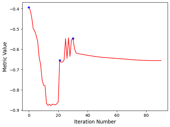

Always remember to query why the optimizer terminated. This will help you understand whether termination is too early, either due to thresholds being too tight, early termination due to small number of iterations - numberOfIterations, or too loose, early termination due to large value for minimal change in similarity measure - convergenceMinimumValue.

PYTHON

print('Final metric value: {0}'.format(registration_method.GetMetricValue()))
print('Optimizer\'s stopping condition, {0}'.format(registration_method.GetOptimizerStopConditionDescription()))

OUTPUT

Final metric value: -0.6561600032169457
Optimizer's stopping condition, GradientDescentOptimizerv4Template: Convergence checker passed at iteration 61.

Now we can visually inspect the results:

PYTHON

moving_resampled = sitk.Resample(moving_image, fixed_image, final_transform, sitk.sitkLinear, 0.0, moving_image.GetPixelID())

interact(
    display_images_with_alpha,
    image_z = (0,fixed_image.GetSize()[2]-1),
    alpha = (0.0,1.0,0.05),
    fixed = fixed(fixed_image),
    moving = fixed(moving_resampled))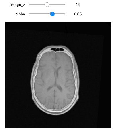

PYTHON

print(f"Origin for fixed image: {fixed_image.GetOrigin()}, shifted moving image: {moving_resampled.GetOrigin()}")
print(f"Spacing for fixed image: {fixed_image.GetSpacing()}, shifted moving image: {moving_resampled.GetSpacing()}")
print(f"Size for fixed image: {fixed_image.GetSize()}, shifted moving image: {moving_resampled.GetSize()}")

OUTPUT

Origin for fixed image: (0.0, 0.0, 0.0), shifted moving image: (0.0, 0.0, 0.0)
Spacing for fixed image: (0.653595, 0.653595, 4.0), shifted moving image: (0.653595, 0.653595, 4.0)
Size for fixed image: (512, 512, 29), shifted moving image: (512, 512, 29)

If we are satisfied with the results, save them to file.

PYTHON

sitk.WriteImage(moving_resampled, os.path.join(OUTPUT_DIR, 'RIRE_training_001_mr_T1_resampled.mha'))
sitk.WriteTransform(final_transform, os.path.join(OUTPUT_DIR, 'RIRE_training_001_CT_2_mr_T1.tfm'))

Segmentation

---

Image segmentation filters process images by dividing them into meaningful regions. SITK provides a wide range of filters to support classical segmentation algorithms, including various thresholding methods and watershed algorithms. The output is typically an image where different integers represent distinct objects, with 0 often used for the background and 1 (or sometimes 255) for foreground objects. After segmenting the data, SITK allows for efficient post-processing, such as labeling distinct objects and analyzing their shapes.

Let’s start by reading in a T1 MRI scan, on which we will perform segmentation operations.

PYTHON

%matplotlib inline
import matplotlib.pyplot as plt
from ipywidgets import interact, fixed
import SimpleITK as sitk

img_T1 = sitk.ReadImage("data/sitk/A1_grayT1.nrrd")
# To visualize the labels image in RGB with needs a image with 0-255 range
img_T1_255 = sitk.Cast(sitk.RescaleIntensity(img_T1), sitk.sitkUInt8)

# Callback invoked by the interact IPython method for scrolling through the image stacks of
# a volume image
def display_images(image_z, npa, title):
    plt.imshow(npa[image_z,:,:], cmap=plt.cm.Greys_r)
    plt.title(title)
    plt.axis('off')
    plt.show()

interact(
    display_images,
    image_z = (0,img_T1.GetSize()[2]-1),
    npa = fixed(sitk.GetArrayViewFromImage(img_T1)),
    title = fixed('Z slices'))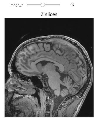

Thresholding

Thresholding is the most basic form of segmentation. It simply labels the pixels of an image based on the intensity range without respect to geometry or connectivity.

PYTHON

# Basic thresholding
seg = img_T1>200
seg_img = sitk.LabelOverlay(img_T1_255, seg)

interact(
    display_images,
    image_z = (0,img_T1.GetSize()[2]-1),
    npa = fixed(sitk.GetArrayViewFromImage(seg_img)),
    title = fixed("Basic thresholding"))

Another example using BinaryThreshold:

PYTHON

# Binary thresholding
seg = sitk.BinaryThreshold(img_T1, lowerThreshold=100, upperThreshold=400, insideValue=1, outsideValue=0)
seg_img = sitk.LabelOverlay(img_T1_255, seg)

interact(
    display_images,
    image_z = (0,img_T1.GetSize()[2]-1),
    npa = fixed(sitk.GetArrayViewFromImage(seg_img)),
    title = fixed("Binary thresholding"))****

ITK has a number of histogram based automatic thresholding filters including Huang, MaximumEntropy, Triangle, and the popular Otsu’s method (OtsuThresholdImageFilter). These methods create a histogram then use a heuristic to determine a threshold value.

PYTHON

# Otsu Thresholding
otsu_filter = sitk.OtsuThresholdImageFilter()
otsu_filter.SetInsideValue(0)
otsu_filter.SetOutsideValue(1)
seg = otsu_filter.Execute(img_T1)
seg_img = sitk.LabelOverlay(img_T1_255, seg)

interact(
    display_images,
    image_z = (0,img_T1.GetSize()[2]-1),
    npa = fixed(sitk.GetArrayViewFromImage(seg_img)),
    title = fixed("Otsu thresholding"))

print(otsu_filter.GetThreshold() )

OUTPUT

236.40869140625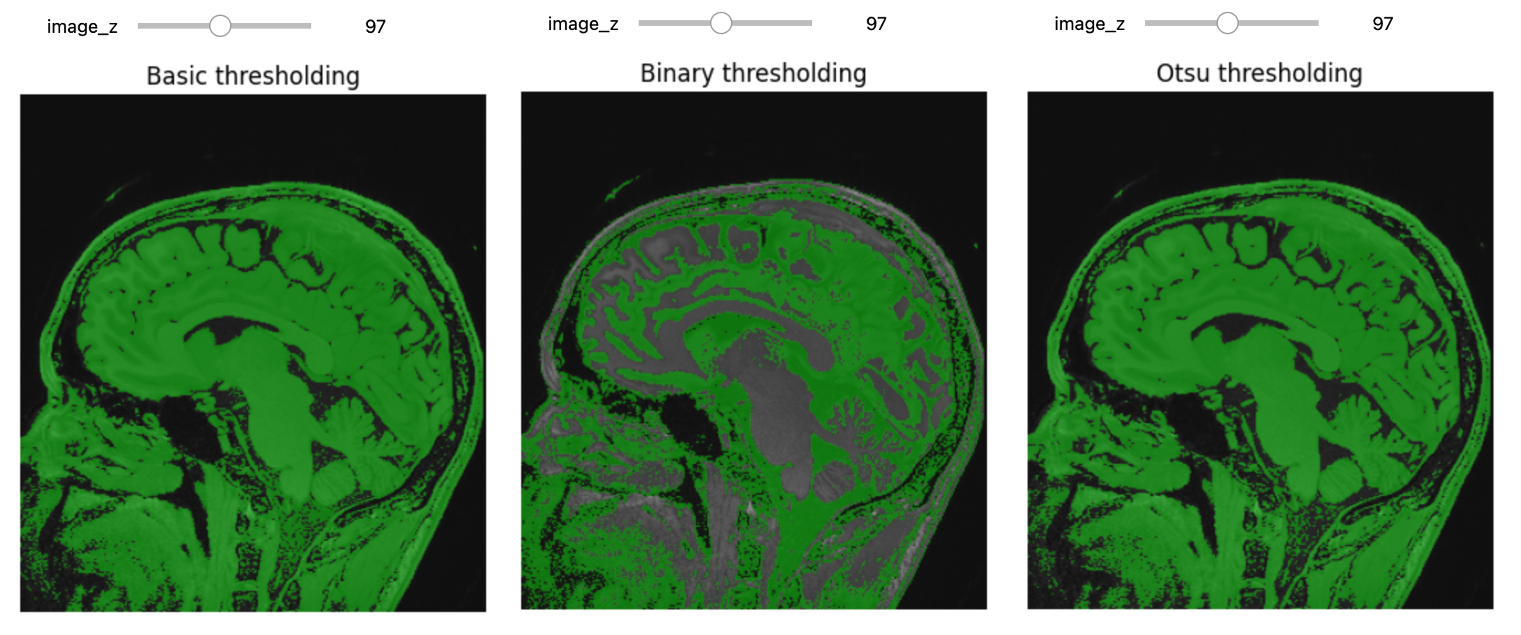

Region Growing Segmentation

The first step of improvement upon the naive thresholding is a class of algorithms called region growing. The common theme for all these algorithms is that a voxel’s neighbor is considered to be in the same class if its intensities are similar to the current voxel. The definition of similar is what varies:

• ConnectedThreshold: The neighboring voxel’s intensity is within explicitly specified thresholds.
• ConfidenceConnected: The neighboring voxel’s intensity is within the implicitly specified bounds \(\mu \pm c \sigma\), where \(\mu\) is the mean intensity of the seed points, \(\sigma\) their standard deviation and \(c\) a user specified constant.
• VectorConfidenceConnected: A generalization of the previous approach to vector valued images, for instance multi-spectral images or multi-parametric MRI. The neighboring voxel’s intensity vector is within the implicitly specified bounds using the Mahalanobis distance \(\sqrt{(x-\mu)^{T\sum{-1}}(x-\mu)}<c\), where \(\mu\) is the mean of the vectors at the seed points, \(\sum\) is the covariance matrix and \(c\) is a user specified constant.
• NeighborhoodConnected

Let’s imagine that we have to segment the left lateral ventricle of the brain image we just visualized.

3D Slicer was used to determine that index: (132,142,96) was a good seed for the left lateral ventricle. Let’s first visualize the seed:

PYTHON

# Initial seed
seed = (132,142,96)
seg = sitk.Image(img_T1.GetSize(), sitk.sitkUInt8)
seg.CopyInformation(img_T1)
seg[seed] = 1
seg = sitk.BinaryDilate(seg, [3]*seg.GetDimension())
seg_img = sitk.LabelOverlay(img_T1_255, seg)

interact(
    display_images,
    image_z = (0,img_T1.GetSize()[2]-1),
    npa = fixed(sitk.GetArrayViewFromImage(seg_img)),
    title = fixed("Initial seed"))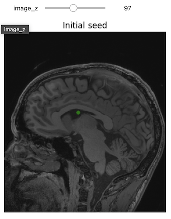

Let’s use ConnectedThreshold functionality:

PYTHON

# Connected Threshold
seg = sitk.ConnectedThreshold(img_T1, seedList=[seed], lower=100, upper=190)

seg_img = sitk.LabelOverlay(img_T1_255, seg)

interact(
    display_images,
    image_z = (0,img_T1.GetSize()[2]-1),
    npa = fixed(sitk.GetArrayViewFromImage(seg_img)),
    title = fixed("Connected threshold"))

Improving upon this is the ConfidenceConnected filter, which uses the initial seed or current segmentation to estimate the threshold range.

This region growing algorithm allows the user to implicitly specify the threshold bounds based on the statistics estimated from the seed points, \(\mu \pm c\sigma\). This algorithm has some flexibility which you should familiarize yourself with:

• The “multiplier” parameter is the constant \(c\) from the formula above.
• You can specify a region around each seed point “initialNeighborhoodRadius” from which the statistics are estimated, see what happens when you set it to zero.
• The “numberOfIterations” allows you to rerun the algorithm. In the first run the bounds are defined by the seed voxels you specified, in the following iterations \(\mu\) and \(\sigma\) are estimated from the segmented points and the region growing is updated accordingly.

PYTHON

seg = sitk.ConfidenceConnected(img_T1, seedList=[seed],
                                   numberOfIterations=0,
                                   multiplier=2,
                                   initialNeighborhoodRadius=1,
                                   replaceValue=1)

seg_img = sitk.LabelOverlay(img_T1_255, seg)

interact(
    display_images,
    image_z=(0,img_T1.GetSize()[2]-1),
    npa = fixed(sitk.GetArrayViewFromImage(seg_img)),
    title=fixed("Confidence connected"))

Since we have available also another MRI scan of the same patient, T2-weighted, we can try to further improve the segmentation. We first load a T2 image from the same person and combine it with the T1 image to create a vector image. This region growing algorithm is similar to the previous one, ConfidenceConnected, and allows the user to implicitly specify the threshold bounds based on the statistics estimated from the seed points. The main difference is that in this case we are using the Mahalanobis and not the intensity difference.

PYTHON

img_T2 = sitk.ReadImage("data/sitk/A1_grayT2.nrrd")
img_multi = sitk.Compose(img_T1, img_T2)
seg = sitk.VectorConfidenceConnected(img_multi, seedList=[seed],
                                             numberOfIterations=1,
                                             multiplier=2.5,
                                             initialNeighborhoodRadius=1)
seg_img = sitk.LabelOverlay(img_T1_255, seg)

interact(
    display_images,
    image_z = (0,img_T1.GetSize()[2]-1),
    npa = fixed(sitk.GetArrayViewFromImage(seg_img)),
    title = fixed("Vector confidence connected"))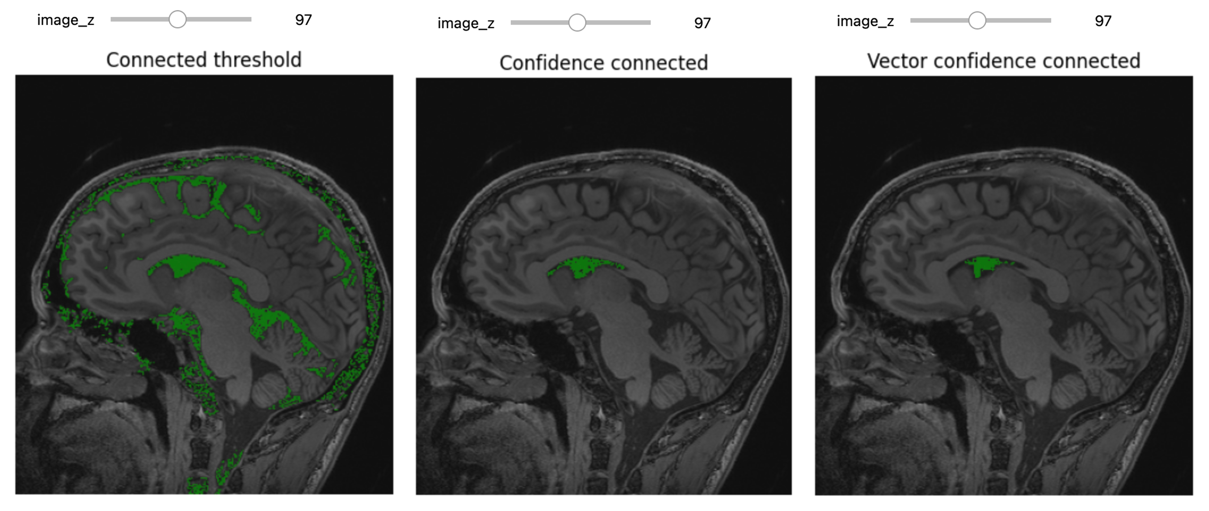

Clean Up

Use of low level segmentation algorithms such as region growing is often followed by a clean up step. In this step we fill holes and remove small connected components. Both of these operations are achieved by using binary morphological operations, opening (BinaryMorphologicalOpening) to remove small connected components and closing (BinaryMorphologicalClosing) to fill holes.

SITK supports several shapes for the structuring elements (kernels) including:

• sitkAnnulus
• sitkBall
• sitkBox
• sitkCross

The size of the kernel can be specified as a scalar (same for all dimensions) or as a vector of values, size per dimension.

The following code cell illustrates the results of such a clean up, using closing to remove holes in the original segmentation.

PYTHON

seg = sitk.ConfidenceConnected(img_T1, seedList=[seed],
                                   numberOfIterations=0,
                                   multiplier=2,
                                   initialNeighborhoodRadius=1,
                                   replaceValue=1)

vectorRadius=(1,1,1)
kernel=sitk.sitkBall
seg_clean = sitk.BinaryMorphologicalClosing(seg, vectorRadius, kernel)
seg_img_clean = sitk.LabelOverlay(img_T1_255, seg_clean)

interact(
    display_images,
    image_z = (0,img_T1.GetSize()[2]-1),
    npa = fixed(sitk.GetArrayViewFromImage(seg_img_clean)),
    title = fixed("Confidence connected after morphological closing"))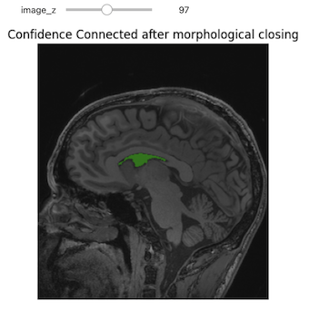

Level-Set Segmentation

There are a variety of level-set based segmentation filter available in ITK:

• GeodesicActiveContour
• ShapeDetection
• ThresholdSegmentation
• LaplacianSegmentation
• ScalarChanAndVese

There is also a modular Level-set framework which allows composition of terms and easy extension in C++.

First we create a label image from our seed.

PYTHON

seed = (132,142,96)

seg = sitk.Image(img_T1.GetSize(), sitk.sitkUInt8)
seg.CopyInformation(img_T1)
seg[seed] = 1
seg = sitk.BinaryDilate(seg, [3]*seg.GetDimension())

Use the seed to estimate a reasonable threshold range.

PYTHON

stats = sitk.LabelStatisticsImageFilter()
stats.Execute(img_T1, seg)

factor = 3.5
lower_threshold = stats.GetMean(1)-factor*stats.GetSigma(1)
upper_threshold = stats.GetMean(1)+factor*stats.GetSigma(1)
print(lower_threshold,upper_threshold)

OUTPUT

81.25184541308809 175.0084466827569

PYTHON

init_ls = sitk.SignedMaurerDistanceMap(seg, insideIsPositive=True, useImageSpacing=True)
lsFilter = sitk.ThresholdSegmentationLevelSetImageFilter()
lsFilter.SetLowerThreshold(lower_threshold)
lsFilter.SetUpperThreshold(upper_threshold)
lsFilter.SetMaximumRMSError(0.02)
lsFilter.SetNumberOfIterations(1000)
lsFilter.SetCurvatureScaling(.5)
lsFilter.SetPropagationScaling(1)
lsFilter.ReverseExpansionDirectionOn()
ls = lsFilter.Execute(init_ls, sitk.Cast(img_T1, sitk.sitkFloat32))
print(lsFilter)

OUTPUT

itk::simple::ThresholdSegmentationLevelSetImageFilter
  LowerThreshold: 81.2518
  UpperThreshold: 175.008
  MaximumRMSError: 0.02
  PropagationScaling: 1
  CurvatureScaling: 0.5
  NumberOfIterations: 1000
  ReverseExpansionDirection: 1
  ElapsedIterations: 119
  RMSChange: 0.0180966
  Debug: 0
  NumberOfThreads: 10
  NumberOfWorkUnits: 0
  Commands: (none)
  ProgressMeasurement: 0.119
  ActiveProcess: (none)

PYTHON

seg_img = sitk.LabelOverlay(img_T1_255, ls>0)

interact(
    display_images,
    image_z = (0,img_T1.GetSize()[2]-1),
    npa = fixed(sitk.GetArrayViewFromImage(seg_img)),
    title = fixed("Level set segmentation"))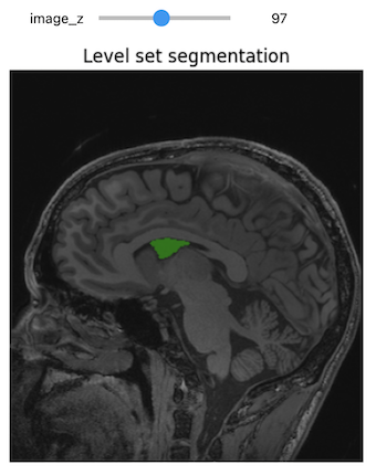

Challenge: Segment on the y-Axis

Try to segment the lateral ventricle using volume’s slices on y-axis instead of z-axis.

Hint: Start by editing the display_images function in order to select the slices on the y-axis.

Show me the solution

PYTHON

def display_images(image_y, npa, title):
    plt.imshow(npa[:,image_y,:], cmap=plt.cm.Greys_r)
    plt.title(title)
    plt.axis('off')
    plt.show()

# Initial seed; we can reuse the same used for the z-axis slices
seed = (132,142,96)
seg = sitk.Image(img_T1.GetSize(), sitk.sitkUInt8)
seg.CopyInformation(img_T1)
seg[seed] = 1
seg = sitk.BinaryDilate(seg, [3]*seg.GetDimension())
seg_img = sitk.LabelOverlay(img_T1_255, seg)

interact(
    display_images,
    image_y = (0,img_T1.GetSize()[2]-1),
    npa = fixed(sitk.GetArrayViewFromImage(seg_img)),
    title = fixed("Initial seed"))

After some attempts, this was the method that gave the best segmentation results:

PYTHON

seed = (132,142,96)

seg = sitk.Image(img_T1.GetSize(), sitk.sitkUInt8)
seg.CopyInformation(img_T1)
seg[seed] = 1
seg = sitk.BinaryDilate(seg, [3]*seg.GetDimension())

stats = sitk.LabelStatisticsImageFilter()
stats.Execute(img_T1, seg)

factor = 3.5
lower_threshold = stats.GetMean(1)-factor*stats.GetSigma(1)
upper_threshold = stats.GetMean(1)+factor*stats.GetSigma(1)
print(lower_threshold,upper_threshold)

init_ls = sitk.SignedMaurerDistanceMap(seg, insideIsPositive=True, useImageSpacing=True)
lsFilter = sitk.ThresholdSegmentationLevelSetImageFilter()
lsFilter.SetLowerThreshold(lower_threshold)
lsFilter.SetUpperThreshold(upper_threshold)
lsFilter.SetMaximumRMSError(0.02)
lsFilter.SetNumberOfIterations(1000)
lsFilter.SetCurvatureScaling(.5)
lsFilter.SetPropagationScaling(1)
lsFilter.ReverseExpansionDirectionOn()
ls = lsFilter.Execute(init_ls, sitk.Cast(img_T1, sitk.sitkFloat32))

OUTPUT

81.25184541308809 175.0084466827569

PYTHON

seg_img = sitk.LabelOverlay(img_T1_255, ls>0)

interact(
    display_images,
    image_y = (0,img_T1.GetSize()[2]-1),
    npa = fixed(sitk.GetArrayViewFromImage(seg_img)),
    title = fixed("Level set segmentation"))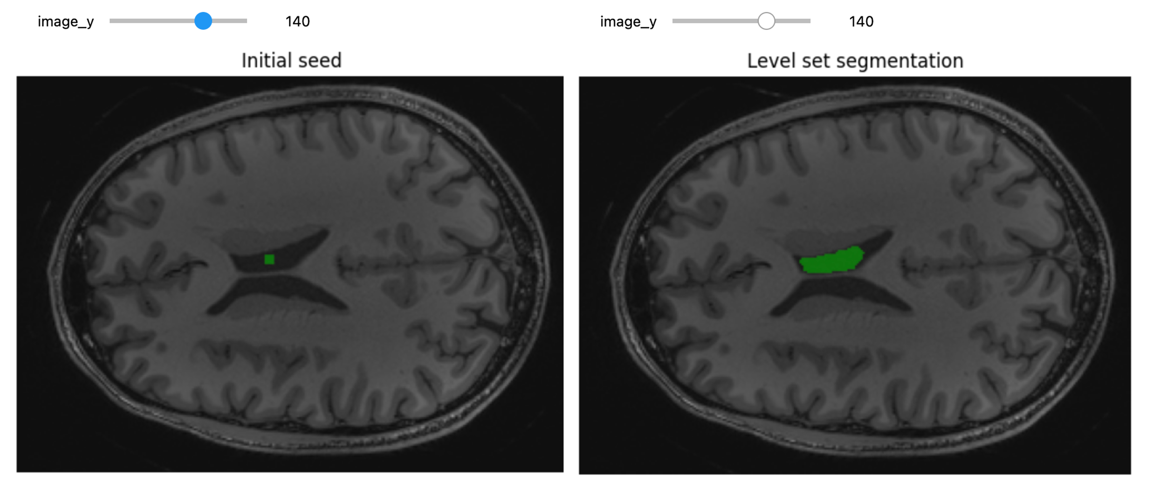

Segmentation Evaluation

Evaluating segmentation algorithms typically involves comparing your results to reference data.

In the medical field, reference data is usually created through manual segmentation by an expert. When resources are limited, a single expert might define this data, though this is less than ideal. If multiple experts contribute, their inputs can be combined to produce reference data that more closely approximates the elusive “ground truth.”

For detailed coding examples on segmentation evaluation, refer to this notebook.

Acknowledgements

---

This episode was largely inspired by the official SITK tutorial, which is copyrighted by NumFOCUS and distributed under the Creative Commons Attribution 4.0 International License, and SITK Notebooks.

Additional Resources

To really understand the structure of SITK images and how to work with them, we recommend some hands-on interaction using the SITK Jupyter notebooks from the SITK official channels. More detailed information about SITK fundamental concepts can also be found here.

Code illustrating various aspects of the registration and segmentation framework can be found in the set of examples which are part of the SITK distribution and in the SITK Jupyter notebook repository.

Key Points

• Registration aligns images for data merging or temporal tracking, while segmentation identifies objects within images, which is critical for detailed analysis.
• SITK simplifies segmentation, registration, and advanced analysis tasks using ITK algorithms and supporting several programming languages.
• Images in SITK are defined by physical space, unlike array-based libraries, ensuring accurate spatial representation and metadata management.
• SITK offers global and bounded domain transformations for spatial manipulation and efficient resampling techniques with various interpolation options.
• Use SITK’s robust capabilities for registration and classical segmentation methods such as thresholding and region growth, ensuring efficient analysis of medical images.