All in One View
Content from Getting Started
Last updated on 2025-01-14 | Edit this page
Estimated time: 50 minutes
Overview
Questions
- Why should I use Julia?
- How do I get started with Julia?
Objectives
- Start a REPL
- Run lines from VS Code
Julia is easy to get into because it centers around a few easy to
understand core concepts: functions, multiple-dispatch, array
polymorphism. It is easy to get needlessly stranded into complications
that hinder the pacing of this lesson. For example: when explaining
for loops you may spend ten minutes explaining all the
finesse of break and continue, but most people
will either know or don’t care. There are several ways to fill these
gaps in the material:
- Explain these concepts when they naturally arise in an example or exercise.
- Point to their existence in a call-out, but refer interested readers to the relevant section in the Julia manual, to study in their own time.
- Give them as part of an exercise: let participants read a section of the manual before solving the exercise. This should empower them to look for the manual when solving their own problems.
This way, you can move on in a natural pacing, only showing the core concepts relevant to the Julia language, and get to interesting (and motivating) challenges earlier in the lesson.
You may want to explain this general strategy to participants before starting on the main content. This will build both patience and trust with your audience.
Why Julia
Most of the participants will be coming from Python, Matlab or a lower level language like C/C++ or Fortran. Why should you be interested in learning Julia?
Performance and usability
Julia promises:
- Native performance: close to or sometimes even exceeding C++ or Fortran.
- Solve the multiple language issue: one language for everything (including GPU).
- As easy to get into as Python or R.
- Designed for parallel computing.
These promises seem tantalizing and are in part what draws people to Julia, but in practice getting into Julia and writing performant code are two different things. Julia has its own idiosyncrasies that need to be understood to really squeeze every erg of performance out of your system.
Julia obtains its performance from being a Just-In-Time (JIT) compiler, on top of the lLVM compiler stack (similar to how Python’s Numba operates).
Language intrinsics
Next to being performant, it turns out that Julia is a very nice language that does some things a bit different from what you may be used to:
- First-class arrays and Broadcasting: arrays, slicing and operating on arrays have dedicated syntax, similar to Matlab.
- Multiple dispatch: Julia functions can be specialized on the entire call signature (not just its first argument like in Object Oriented Programming).
- Macros and Meta-programming: The Just-in-time nature of the Julia compiler exposes a wide range of meta-programming capabilities, ranging from small macros to enhance the expressibility of the language to full-on code generation.
Meta-programming, while very powerful, is also very easy to abuse, often leading to unreadable non-idiomatic code. So tread with care! We’ll see some examples where macros are indispensable though, and the SciML stack relies deeply on on-the-fly code-generation.
Why are you interested in Julia? What is your current go-to for efficient computing?
Running Julia
When working in Julia it is very common to do so from the REPL (Read-Eval-Print Loop). Please open the Julia REPL on your system
OUTPUT
$ julia
               _
   _       _ _(_)_     |  Documentation: https://docs.julialang.org
  (_)     | (_) (_)    |
   _ _   _| |_  __ _   |  Type "?" for help, "]?" for Pkg help.
  | | | | | | |/ _` |  |
  | | |_| | | | (_| |  |  Version 1.10.3 (2024-04-30)
 _/ |\__'_|_|_|\__'_|  |  Official https://julialang.org/ release
|__/                   |

julia>
The REPL needs a small introduction since it has several modes.
| Key | Prompt | Mode |
|---|---|---|
| None | julia> |
Standard Julia input. |
] |
pkg> |
Pkg mode. Commands entered here are functions in
the Pkg module. |
; |
shell> |
Shell mode. |
? |
help?> |
Help mode. Type the name of any entity to look up its documentation. |
Play with the REPL (5min)
-
Pkgmode has ahelpcommand to help you along. Find out what theaddcommand does. - Check the contents of the folder in which your are running your REPL
(
lson Unix,diron Windows). - Find out what the
printmethod does in Julia.
-
]help add, theaddcommand installs packages ;ls?print
Pluto
Pluto is the notebook environment from which we will teach much of this workshop. We can run it from the Julia REPL.
OUTPUT
pkg> add Pluto
... quite a bit of output ...

julia> using Pluto

julia> Pluto.run()
[ Info: Loading...
┌ Info:
└ Opening http://localhost:1235/?secret=xyzxyzxyz in your default browser... ~ have fun!
┌ Info:
│ Press Ctrl+C in this terminal to stop Pluto
└
VS Code
VS Code is the editor for which Julia has the best support. We’ll be
needing to run Julia in multiple threads later on, so we’ll set some
arguments for the REPL in settings.json (press
Ctrl-,).
Now when you start a new REPL, (Ctrl-Shift-P, search
“Julia REPL”) you can query the number of threads available:
Julia as a calculator (5min)
Try to play around in Pluto to use Julia as a calculator.
- What do you find is the operator for exponentiation?
- How do you assign a variable?
- What happens when you divide any two integers? Use the
typeoffunction to inspect the type of the result. Can you figure out how to integer division (search the documentation!)? - What happens in Pluto when you change a variable that is depended upon?
- In Julia exponentiation is
^. - Just like you’re used to
x = 3. - The
/operator always returns a floating point value. To get to integer division, we want the÷operator, which can be typed using\divand then press TAB. Or you can use the equivalentdivfunction. - Pluto updates all dependent computations automatically. This is known as a reactive notebook.
- In Julia, the REPL is much more important than in some other languages.
- Pluto is a reactive environment
- VS Code has the best editor integration for Julia
Activate the Workshop Environment
For this workshop, we prepared an environment. Press ]
in the REPL to activate Pkg mode. Make sure that you are in
the path where you prepared your environment (see Setup
Instructions).
(v1.11) pkg> activate .
(EfficientJulia) pkg>
Alternatively, check the little “Julia env” message at the bottom of VS Code, and make sure that the correct environment is there.
You should now be able to generate a plot using GLMakie
(that one dependency that made you wait)
JULIA
using GLMakie
x = -3.0:0.1:3.0
z = sinc.(sqrt.(x.^2 .+ x'.^2))
surface(x, x, z, alpha=0.5)
wireframe!(x, x, z, color=:black, linewidth=0.5)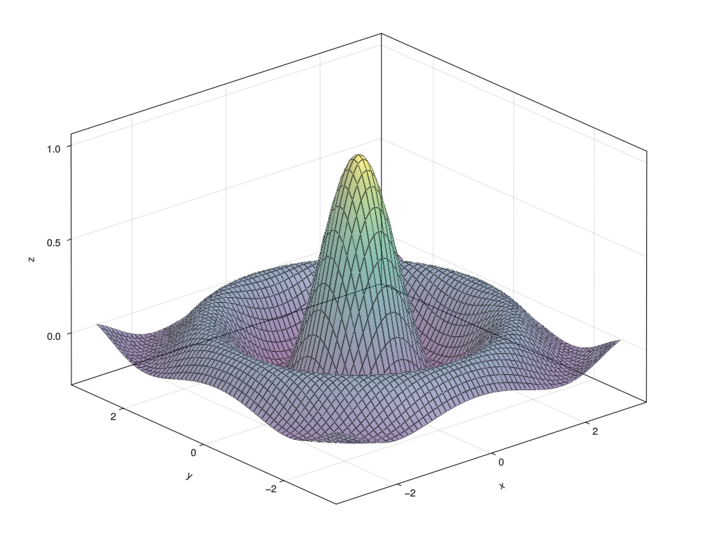
To create the above figure:
JULIA
#| classes: ["task"]
#| creates: episodes/fig/getting-started-makie.png
#| collect: figures

module Script
using GLMakie

function main()
    x = -3.0:0.1:3.0
    z = sinc.(sqrt.(x.^2 .+ x'.^2))

    fig = Figure(size=(1024, 768))
    ax = Axis3(fig[1,1])
    surface!(ax, x, x, z, alpha=0.5)
    wireframe!(ax, x, x, z, color=:black, linewidth=0.5)
    save("episodes/fig/getting-started-makie.png", fig)
end
end

Script.main()
Content from Introduction to Julia
Last updated on 2025-01-14 | Edit this page
Overview
Questions
- How do I write elementary programs in Julia?
- What are the differences with Python/Matlab/R?
Objectives
- functions
- loops
- conditionals
- scoping
Unfortunately, it lies outside the scope of this workshop to give a introduction to the full Julia language. Instead, we’ll briefly show the basic syntax, and then focus on some key differences with other popular languages.
Much of the content of the lesson relies on “Show, don’t tell”. This introduction feels far from complete, but that’s Ok. It is just enough to teach the forms of function definitions, and some peculiarities that might trip-up people that are used to a different language:
About Julia
These are some words that we will write down: never forget.
- A Just-in-time compiled, dynamically typed language
- multiple dispatch
- expression based syntax
- rich macro system
Oddities for Pythonistas:
- 1-based indexing
- lexical scoping
Eval
How is Julia evaluated? Types only instantiate at run-time, triggering the compile time specialization of untyped functions.
- Julia can be “easy”, because the user doesn’t have to tinker with types.
- Julia can be “fast”, as soon as the compiler knows all the types.
When a function is called with a hitherto new type signature, compilation is triggered. Julia’s biggest means of abstraction: multiple dispatch is only an emergent property of this evaluation strategy.
Julia has a herritage from functional programming languages (nowadays well hidden not to scare people). What we get from this:
- expression based syntax: everything is an expression, meaning it reduces to a value
- a rich macro system: we can extend the language itself to suit our needs (not covered in this workshop)
Julia is designed to replace Matlab:
- high degree of built-in support for multi-dimensional arrays and linear algebra
- ecosystem of libraries around numeric modelling
Julia is designed to replace Fortran:
- high performance
- accellerate using
Threadsor of the GPU interfaces - scalable through
DistributedorMPI
Julia is designed to replace Conda:
- quality package system with pre-compiled binary libraries for system dependencies
- highly reproducible
- easy to use on HPC facilities
Julia is not (some people might get angry for this):
- a suitable scripting language
- a systems programming language like C or Rust (imagine waiting for
lsto compile every time you run it) - replacing either C or Python anytime soon
Functions
Functions are declared with the function keyword. The
block or function body is ended with
end. All blocks in Julia end with end.
Let’s compute the force between Earth and Moon, given the following constants:
JULIA
const EARTH_MASS = 5.97219e24
const LUNAR_MASS = 7.34767e22
const LUNAR_DISTANCE = 384_400_000.0OUTPUT
1.982084770423259e26There is a shorter syntax for functions that is useful for one-liners:
Anonymous functions (or lambdas)
Julia inherits a lot of concepts from functional programming. There are two ways to define anonymous functions:
And a shorter syntax,
Higher order functions
Use the map function in combination with an anonymous
function to compute the squares of the first ten integers (use
1:10 to create that range).
If statements, for loops
Here’s another function that’s a little more involved.
JULIA
function is_prime(x)
  if x < 2
    return false
  end

  for i = 2:isqrt(x)
    if x % i == 0
      return false
    end
  end

  return true
endRanges
The for loop iterates over the range
2:isqrt(x). We’ll see that Julia indexes sequences starting
at integer value 1. This usually implies that ranges are
given inclusive on both ends: for example, collect(3:6)
evaluates to [3, 4, 5, 6].
Challenge
The i == j && continue is a short-cut notation
for
We could also have written i != j || continue.
In general, the || and && operators
can be chained to check increasingly stringent tests. For example:
Here, the second condition can only be evaluated if the first one was true.
Rewrite the is_prime function using this
notation.
Return statement
In Julia, the return statement is not always strictly
necessary. Every statement is an expression, meaning that it has a
value. The value of a compound block is simply that of its last
expression. In the above function however, we have a non-local return:
once we find a divider for a number, we know the number is not prime,
and we don’t need to check any further.
Many people find it more readable however, to always have an explicit
return.
The fact that the return statement is optional for
normal function exit is part of a larger philosophy: everything is an
expression.
More on for-loops
Loop iterations can be skipped using continue, or broken
with break, identical to C or Python.
Lexical scoping
Julia is lexically scoped. This means that variables do not outlive the block that they’re defined in. In a nutshell, this means the following:
OUTPUT
42
1
2
3
42
In effect, the variable s inside the for-loop is said to
shadow the outer definition. Here, we also see a first
example of a let binding, creating a scope for some
temporary variables to live in.
Loops and conditionals
Write a loop that prints out all primes below 100.
Some important first lessons
- Always enclose code in functions because functions are compiled
- Don’t use global mutable variables
- Julia has
if-else,for,while,functionandmoduleblocks that are not dissimilar from other languages. - Blocks are all ended with
end. - …
- Julia variables are not visible outside the block in which they’re defined (unlike Python).
Content from Types and Dispatch
Last updated on 2025-01-12 | Edit this page
Overview
Questions
- How does Julia deal with types?
- Can I do Object Oriented Programming?
- People keep talking about multiple dispatch. What makes it so special?
Objectives
- dispatch
- structs
- abstract types
Parametric types will only be introduced when the occasion arises.
Julia is a dynamically typed language. Nevertheless, we will see that knowing where and where not to annotate types in your program is crucial for managing performance.
In Julia there are two reasons for using the type system:
- structuring your data by declaring a
struct - dispatching methods based on their argument types
Inspection
You may inspect the dynamic type of a variable or expression using
the typeof function. For instance:
OUTPUT
Int64OUTPUT
String(plenary) Types of floats
Check the type of the following values:
33.146.62607015e-346.6743f-116e0 * 7f0
Int64Float64Float64Float32Float64
Structures
Multiple dispatch (function overloading)
OUTPUT
Point2(0, 1)OOP (Sort of)
Julia is not an Object Oriented language. If you feel the unstoppable urge to implement a class-like abstraction, this can be done through abstract types.
- Julia is fundamentally a dynamically typed language.
- Static types are only ever used for dispatch.
- Multiple dispatch is the most important means of abstraction in Julia.
- Parametric types are important to achieve type stability.
Content from Simulating the Solar System
Last updated on 2025-01-14 | Edit this page
Overview
Questions
- How can I work with physical units?
- How do I quickly visualize some data?
- How is dispatch used in practice?
Objectives
- Learn to work with
Unitful - Take the first steps with
Makiefor visualisation - Work with
const - Define a
struct
In this episode we’ll be building a simulation of the solar system. That is, we’ll only consider the Sun, Earth and Moon, but feel free to add other planets to the mix later on! To do this we need to work with the laws of gravity. We will be going on extreme tangents, exposing interesting bits of the Julia language as we go.
Introduction to Unitful
We’ll be using the Unitful library to ensure that we
don’t mix up physical units.
Using Unitful is without any run-time overhead. The unit
information is completely contained in the Quantity type.
With Unitful we can attach units to quantities using the
@u_str syntax:
Try adding incompatible quantities
For instance, add a quantity in meters to one in seconds. Be creative. Can you understand the error messages?
Next to that, we use the Vec3d type from
GeometryBasics to store vector particle positions.
Libraries in Julia tend to work well together, even if they’re not
principally designed to do so. We can combine Vec3d with
Unitful with no problems.
Generate random Vec3d
The Vec3d type is a static 3-vector of double precision
floating point values. Read the documentation on the randn
function. Can you figure out a way to generate a random
Vec3d?
Two bodies of mass \(M\) and \(m\) attract each other with the force
\[F = \frac{GMm}{r^2},\]
where \(r\) is the distance between those bodies, and \(G\) is the universal gravitational constant.
JULIA
#| id: gravity
const G = 6.6743e-11u"m^3*kg^-1*s^-2"
gravitational_force(m1, m2, r) = G * m1 * m2 / r^2
Verify that the force exerted between two 1 million kg bodies at a distance of 2.5 meters is about equal to holding a 1kg object on Earth. Or equivalently two one tonne objects at a distance of 2.5 mm (all of the one tonne needs to be concentrated in a space tiny enough to get two of them at that close a distance)
A better way to write the force would be,
\[\vec{F} = \hat{r} \frac{G M m}{|r|^2},\]
where \(\hat{r} = \vec{r} / |r|\), so in total we get a third power, \(|r|^3 = (r^2)^{3/2}\), where \(r^2\) can be computed with the dot-product.
JULIA
#| id: gravity
gravitational_force(m1, m2, r::AbstractVector) = r * (G * m1 * m2 * (r ⋅ r)^(-1.5))Not all of you will be jumping up and down for doing high-school physics. We will get to other sciences than physics later in this workshop, I promise!
The ⋅ operator (enter using
\cdot<TAB>) performs the
LinearAlgebra.dot function. We could have done
sum(r * r). However, the sum function works on
iterators and has a generic implementation. We could define our own
dot function:
JULIA
function dot(a::AbstractVector{T}, b::AbstractVector{T}) where {T}
    Prod = typeof(zero(T) * zero(T))
	x = zero(Prod)
	@simd ivdep for i in eachindex(a)
		x += a[i] * b[i]
	end
	return x
end
If we look for the source
@which LinearAlgebra.dot(a, b)We find that we’re actually running the dot product from the
StaticArrays library, which has a very similar
implementation as ours.
The zero function
The zero function is overloaded to return a zero object
for any type that has a natural definition of zero.
The one function
The return-value of zero should be the additive identity
of the given type. So for any type T:
There also is the one function which returns the
multiplicative identity of a given type. Try to use the *
operator on two strings. What do you expect one(String) to
return?
Particles
We are now ready to define the Particle type.
JULIA
#| id: gravity
using Unitful: Mass, Length, Velocity
mutable struct Particle
    mass::typeof(1.0u"kg")
    position::typeof(Vec3d(1)u"m")
    momentum::typeof(Vec3d(1)u"kg*m/s")
end

Particle(mass::Mass, position::Vec3{L}, velocity::Vec3{V}) where {L<:Length,V<:Velocity} =
    Particle(mass, position, velocity * mass)

velocity(p::Particle) = p.momentum / p.mass
We store the momentum of the particle, so that what follows is slightly simplified.
It is custom to divide the computation of orbits into a kick
and drift function. (There are deep mathematical reasons for
this that we won’t get into.) We’ll first implement the
kick! function, that updates a collection of particles,
given a certain time step.
The kick
The following function performs the kick! operation on a
set of particles. We’ll go on a little tangent for every line in the
function.
JULIA
#| id: gravity
function kick!(particles, dt)
    for i in eachindex(particles)
        for j in 1:(i-1)
            r = particles[j].position - particles[i].position
            force = gravitational_force(particles[i].mass, particles[j].mass, r)
            particles[i].momentum += dt * force
            particles[j].momentum -= dt * force
        end
    end
    return particles
endWhy the ! exclamation mark?
In Julia it is custom to have an exclamation mark at the end of names of functions that mutate their arguments.
Use eachindex
Note the way we used eachindex. This idiom guarantees
that we can’t make out-of-bounds errors. Also this kind of indexing is
generic over other collections than vectors. However, this is
immediately destroyed by our next loop.
We’re iterating over the range 1:(i-1), and so we don’t
compute forces twice. Momentum should be conserved!
Luckily the drift! function is much easier to implement,
and doesn’t require that we know about all particles.
JULIA
#| id: gravity
function drift!(p::Particle, dt)
    p.position += dt * p.momentum / p.mass
end

function drift!(particles, dt)
    for p in values(particles)
        drift!(p, dt)
    end
    return particles
end
Note that we defined the drift! function twice, for
different arguments. We’re using the dispatch mechanism to write
clean/readable code.
Fixing arguments
One pattern that you can find repeatedly in the standard library is that of fixing arguments of functions to make them more composable. For instance, most comparison operators allow you to give a single argument, saving the second argument for a second invocation.
and even
We can do a similar thing here:
These kinds of identities let us be flexible in how to use and combine methods in different circumstances.
This defines the leap_frog! function as first performing
a kick! and then a drift!. Another way to
compose these functions is the |> operator. In contrast
to the ∘ operator, |> is very popular and
seen everywhere in Julia code bases.
With random particles
Let’s run a simulation with some random particles
JULIA
#| id: gravity
function run_simulation(particles, dt, n)
    result = Matrix{typeof(Vec3d(1)u"m")}(undef, n, length(particles))
    x = deepcopy(particles)
    for c in eachrow(result)
        x = leap_frog!(dt)(x)
        c[:] = [p.position for p in values(x)]
    end
    DataFrame(:time => (1:n)dt, (Symbol.("p", keys(particles)) .=> eachcol(result))...)
end
Frame of reference
We need to make sure that our entire system doesn’t have a net velocity. Otherwise it will be hard to visualize our results!
Plotting
JULIA
#| id: gravity
using DataFrames
using GLMakie

function plot_orbits(orbits::DataFrame)
    fig = Figure()
    ax = Axis3(fig[1, 1], limits=((-5, 5), (-5, 5), (-5, 5)))

    for colname in names(orbits)[2:end]
        scatter!(ax, [orbits[1, colname] / u"m"])
        lines!(ax, orbits[!, colname] / u"m")
    end

    fig
end
Try a few times with two random particles. You may want to use the
set_still! function to negate any collective motion.
JULIA
#| id: gravity
function random_orbits(n, mass)
    random_particle() = Particle(mass, randn(Vec3d)u"m", randn(Vec3d)u"mm/s")
    particles = set_still!([random_particle() for _ in 1:n])
    run_simulation(particles, 1.0u"s", 5000)
end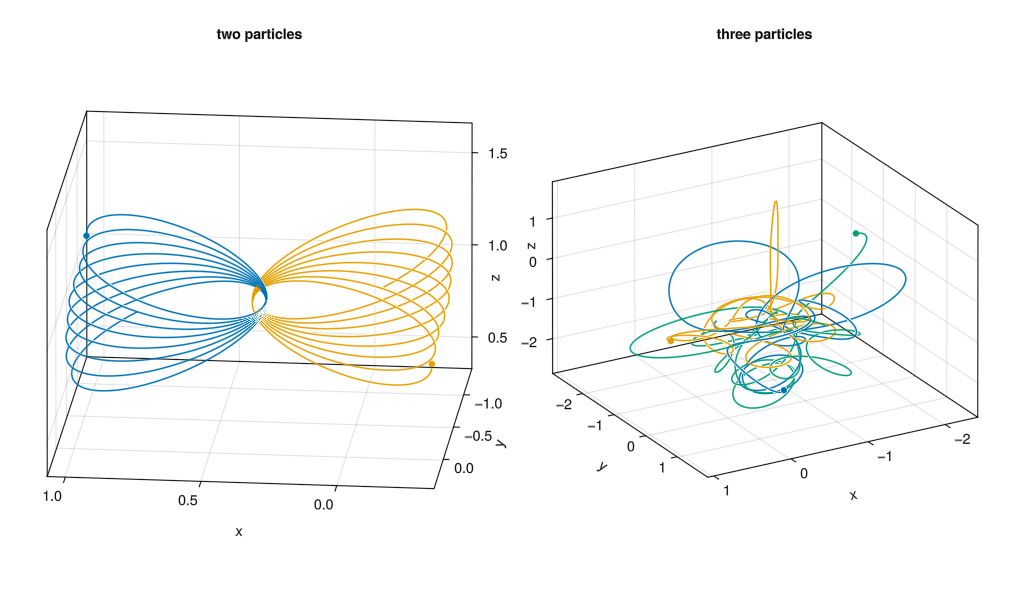
Solar System
JULIA
#| id: gravity
const SUN = Particle(2e30u"kg",
    Vec3d(0.0)u"m",
    Vec3d(0.0)u"m/s")

const EARTH = Particle(6e24u"kg",
    Vec3d(1.5e11, 0, 0)u"m",
    Vec3d(0, 3e4, 0)u"m/s")

const MOON = Particle(7.35e22u"kg",
    EARTH.position + Vec3d(3.844e8, 0.0, 0.0)u"m",
velocity(EARTH) + Vec3d(0, 1e3, 0)u"m/s")Challenge
Plot the orbit of the moon around the earth. Make a
Dataframe that contains all model data, and work from
there. Can you figure out the period of the orbit?
-
Plots.jlis in some ways the ‘standard’ plotting package, but it is in fact quite horrible. -
Makie.jloffers a nice interface, pretty plots, is generally stable and very efficient once things have been compiled.
JULIA
#| file: src/Gravity.jl
module Gravity

using GLMakie
using Unitful
using GeometryBasics
using DataFrames
using LinearAlgebra

<<gravity>>

end
JULIA
#| classes: ["task"]
#| creates: episodes/fig/random-orbits.png
#| collect: figures

module Script

using Unitful
using GLMakie
using DataFrames
using Random
using EfficientJulia.Gravity: random_orbits

function plot_orbits!(ax, orbits::DataFrame)
    for colname in names(orbits)[2:end]
        scatter!(ax, [orbits[1,colname] / u"m"])
        lines!(ax, orbits[!,colname] / u"m")
    end
end

function main()
    Random.seed!(0)
    orbs1 = random_orbits(2, 1e6u"kg")
    Random.seed!(15)
    orbs2 = random_orbits(3, 1e6u"kg")

    fig = Figure(size=(1024, 600))
    ax1 = Axis3(fig[1,1], azimuth=π/2+0.1, elevation=0.1π, title="two particles")
    ax2 = Axis3(fig[1,2], azimuth=π/3, title="three particles")

    plot_orbits!(ax1, orbs1)
    plot_orbits!(ax2, orbs2)

    save("episodes/fig/random-orbits.png", fig)
    fig
end

end

Script.main()
Content from Packages and environments
Last updated on 2025-01-12 | Edit this page
Overview
Questions
- How do I work with environments?
- What are these
Project.tomlandManifest.tomlfiles? - How do I install more dependencies?
Objectives
- pkg> status
- pkg> add (in more details)
- pkg> remove
- Project.toml
- Manifest.toml
- pkg> instantiate
- pkg> activate
- pkg> activate –temp
- pkg> activate @place
- Julia has a built-in package manager called
Pkg. - The package manager is usually accessed from the REPL, by pressing
]. -
Project.tomllists the dependencies of a package. -
Manifest.tomlspecifies a completely reproducible environment with exact versions.
Content from Package development
Last updated on 2025-01-12 | Edit this page
Overview
Questions
- What is the best workflow for developing a Julia package?
- How can I prevent having to recompile every time I make a change?
Objectives
- Quick start with pkg> generate
- Basic structure of a package
- VSCode
- Revise.jl
- Currently, the editor with (by far) the best support is VSCode.
- The
Revise.jlmodule can automatically reload parts of your code that have changed. - Best practice: file names should reflect module names.
Content from Best practices
Last updated on 2025-01-13 | Edit this page
Overview
Questions
- How do I setup unit testing?
- What about documentation?
- Are there good Github Actions available for CI/CD?
- I like autoformatters for my code, what is the best one for Julia?
- How can I make all this a bit easier?
Objectives
- tests
- documentation
- GitHub workflows
- JuliaFormatter.jl
- BestieTemplate.jl
The following is a function for computing the roots of a cubic polynomial
\[ax^3 + bx^2 + cx + d = 0.\]
There is an interesting story about these equations. It was known for a long time how to solve quadratic equations. In 1535 the Italian mathematician Tartaglia discovered a way to solve cubic equations, but guarded his secret carefully. He was later persuaded by Cardano to reveal his secret on the condition that Cardano wouldn’t reveal it further. However, later Cardano found out that an earlier mathematician Scipione del Ferro had also cracked the problem and decided that this anulled his deal with Tartaglia, and published anyway. These days, the formula is known as Cardano’s formula.
The interesting bit is that this method requires the use of complex numbers.
JULIA
function cubic_roots(a, b, c, d)
	cNaN = NaN+NaN*im

	if (a != 0)
		delta0 = b^2 - 3*a*c
		delta1 = 2*b^3 - 9*a*b*c + 27*a^2*d
		cc = ((delta1 + sqrt(delta1^2 - 4*delta0^3 + 0im)) / 2)^(1/3)
		zeta = -1/2 + 1im/2 * sqrt(3)

		k = (0, 1, 2)
		return (-1/(3*a)) .* (b .+ zeta.^k .* cc .+ delta0 ./ (zeta.^k .* cc))
	end

	if (b != 0)
		delta = sqrt(c^2 - 4 * b * d + 0im)
		return ((-c - delta) / (2*b), (-c + delta) / (2*b), cNaN)
	end

	if (c != 0)
		return (-d/c + 0.0im, cNaN, cNaN)
	end

	if (d != 0)
		return (cNaN, cNaN, cNaN)
	end

	return (0.0+0.0im, cNaN, cNaN)
end- Julia has integrated support for unit testing.
-
Documenter.jlis the standard package for generating documentation. - The Julia ecosystem is well equiped to help you keep your code in fit shape.
Content from Julia and performance
Last updated on 2025-01-12 | Edit this page
Overview
Questions
- How can Julia be so much faster than Python?
- I can’t say Julia is slow, but why is it so sluggish?
- How can I reason about performance?
Objectives
- Understand the strategy of JIT compilation.
- The Julia compiler compiles a function once its called with a specific type signature.
Content from Reducing allocations on the Logistic Map
Last updated on 2025-01-13 | Edit this page
Overview
Questions
- How can I reduce the number of allocations?
Objectives
- Apply a code transformation to write to pre-allocated memory.
Logistic growth (in economy or biology) is sometimes modelled using the recurrence formula:
\[N_{i+1} = r N_{i} (1 - N_{i}),\]
also known as the logistic map, where \(r\) is the reproduction factor. For low values of \(N\) this behaves as exponential growth. However, most growth processes will hit a ceiling at some point. Let’s try:
Vary r
Try different values of \(r\), what do you see?
Extra (advanced!): see the Makie
documention on Slider. Can you make an interactive
plot?
JULIA
let
    fig = Figure()
    sl_r = Slider(fig[2, 2], range=1.0:0.001:4.0, startvalue=2.0)
    Label(fig[2,1], lift(r->"r = $r", sl_r.value))
    points = lift(sl_r.value) do r
        take(iterated(logistic_map(r), 0.001), 50) |> collect
    end
    ax = Axis(fig[1, 1:2], limits=(nothing, (0.0, 1.0)))
    plot!(ax, points)
    lines!(ax, points)
    fig
end
There seem to be key values of \(r\) where the iteration of the logistic map splits into periodic orbits, and even get into chaotic behaviour.
We can plot all points for an arbitrary sized orbit for all values of
\(r\) between 2.6 and 4.0. First of
all, let’s see how the iterated |> take |> collect
function chain performs.
JULIA
function iterated_fn(f, x, n)
    result = Float64[]
    for i in 1:n
        x = f(x)
        push!(result, x)
    end
    return result
end

@btime iterated_fn(logistic_map(3.5), 0.5, 10000)
That seems to be slower than the original! Let’s try to improve:
JULIA
function iterated_fn(f, x, n)
    result = Vector{Float64}(undef, n)
    for i in 1:n
        x = f(x)
        result[i] = x
    end
    return result
end

@benchmark iterated_fn(logistic_map(3.5), 0.5, 10000)
We can do better if we don’t need to allocate:
JULIA
function iterated_fn!(f, x, out)
    for i in eachindex(out)
        x = f(x)
        out[i] = x
    end
end

out = Vector{Float64}(undef, 10000)
@benchmark iterated_fn!(logistic_map(3.5), 0.5, out)
JULIA
function logistic_map_points(r::Real, n_skip)
    make_point(x) = Point2f(r, x)
    x0 = nth(iterated(logistic_map(r), 0.5), n_skip)
    Iterators.map(make_point, iterated(logistic_map(r), x0))
end

@btime takestrict(logistic_map_points(3.5, 1000), 1000) |> collect
JULIA
function logistic_map_points(rs::AbstractVector{R}, n_skip, n_take) where {R <: Real}
    Iterators.flatten(Iterators.take(logistic_map_points(r, n_skip), n_take) for r in rs)
end

@benchmark logistic_map_points(LinRange(2.6, 4.0, 1000), 1000, 1000) |> collect
First of all, let’s visualize the output because its so pretty!
JULIA
let
    pts = logistic_map_points_td(LinRange(2.6, 4.0, 10000), 1000, 10000)
	fig = Figure(size=(800, 700))
	ax = Makie.Axis(fig[1,1], limits=((2.6, 4.0), nothing))
	datashader!(ax, pts, async=false, colormap=:deep)
	fig
end
JULIA
function collect!(it, tgt)
    for (i, v) in zip(eachindex(tgt), it)
        tgt[i] = v_map(r) = n -> r
    end
end

function logistic_map_points_td(rs::AbstractVector{R}, n_skip, n_take) where {R <: Real}
    result = Matrix{Point2}(undef, n_take, length(rs))
    # Threads.@threads for i in eachindex(rs)
    for i in eachindex(rs)
        collect!(logistic_map_points(rs[i], n_skip), view(result, :, i))
    end
    return reshape(result, :)
end

@benchmark logistic_map_points_td(LinRange(2.6, 4.0, 1000), 1000, 1000)
@profview logistic_map_points_td(LinRange(2.6, 4.0, 10000), 1000, 1000)Rewrite the logistic_map_points
function
Rewrite the last function, so that everything is in one body (Fortran style!). Is this faster than using iterators?
JULIA
function logistic_map_points_raw(rs::AbstractVector{R}, n_skip, n_take, out::AbstractVector{P}) where {R <: Real, P}
    # result = Array{Float32}(undef, 2, n_take, length(rs))
    # result = Array{Point2f}(undef, n_take, length(rs))
    @assert length(out) == length(rs) * n_take
    # result = reshape(reinterpret(Float32, out), 2, n_take, length(rs))
    result = reshape(out, n_take, length(rs))
    for i in eachindex(rs)
        x = 0.5
        r = rs[i]
        for _ in 1:n_skip
            x = r * x * (1 - x)
        end
        for j in 1:n_take
            x = r * x * (1 - x)
            result[j, i] = P(r, x)
            #result[1, j, i] = r
            #result[2, j, i] = x
        end
        # result[1, :, i] .= r
    end
    # return reshape(reinterpret(Point2f, result), :)
    # return reshape(result, :)
    out
end

out = Vector{Point2d}(undef, 1000000)
logistic_map_points_raw(LinRange(2.6, 4.0, 1000), 1000, 1000, out)
@benchmark logistic_map_points_raw(LinRange(2.6, 4.0, 1000), 1000, 1000, out)- Allocations are slow.
- Growing arrays dynamically induces allocations.
Content from Performance: do's and don'ts
Last updated on 2025-01-12 | Edit this page
Overview
Questions
- Can you give me some guiding principles on how to keep Julia code performant?
Objectives
- Identify potential problems with given code.
Type Stability
A good summary on type stability can be found in the following blog post: - Writing type-stable Julia code
- Don’t use mutable global variables.
- Write your code inside functions.
- Specify element types for containers and structs.
- Specialize functions instead of doing manual dispatch.
- Write functions that always return the same type (type stability).
- Don’t change the type of variables.
Content from Channels and do-syntax
Last updated on 2025-01-12 | Edit this page
Overview
Questions
- How can we manage streams with internal state?
- Does Julia have context managers, or other ways to manage resources?
Objectives
- Work with
Channels to create streams. - Understand
dosyntax.
- Channels are Julia’s primary means of state management and inter-thread communication.
Content from Getting Started
Last updated on 2025-01-12 | Edit this page
Overview
Questions
- How do we distribute work across threads?
Objectives
- Change for-loops to run parallel.
- Launch tasks and generate results asynchronously.
- Basic parallel for-loops are done with the
@threadsmacro. - Julia has built-in support for atomics.
- Channels are primary means of asynchronous communication.
Content from Getting Started
Last updated on 2025-01-12 | Edit this page
Overview
Questions
- Does Julia have support for MPI?
- Can I scale my tasks to multiple machines?
Objectives
- Learn how to run Julia on HPC.
- Julia has built-in support for distributed computing.
Content from Transducers
Last updated on 2025-01-12 | Edit this page
Overview
Questions
- Aren’t there better abstractions to deal with parallelism, like
mapandreduce? - What other libraries exist to aid in parallel computing, and what makes them special?
Objectives
- Exposure to some higher level programming concepts.
- Learn how to work with the pipe
|>operator. - Write performant code that scales.
List of libraries:
Transducers.jlFolds.jlFLoops.jl
- Transducers are composable functions.
- Using the
|>operator can make your code consise, with fewer parenthesis, and more readable. - Overusing the
|>operator can make your code an absolute mess. - Using Tranducers you can build scalable data pipe lines.
- Many Julia libraries for parallel computing and data processing are built on top of Tranducers.
Content from Recommended libraries
Last updated on 2025-01-12 | Edit this page
Overview
Questions
- Is there a recommended set of standard libraries?
- What is the equivalent of SciPy in Julia.
Objectives
- Get street-wise.
This is a nice closing episode.
- SciML toolkit is dominant but not always the best choice.
- Search for libraries that specify your needs.
Content from GPU Programming
Last updated on 2025-01-14 | Edit this page
Overview
Questions
- Can I have some Cuda please?
Objectives
- See what the current state of GPU computing over Julia is.
State of things
There are separate packages for GPU computing, depending on the hardware you have.
| Brand | Lib |
|---|---|
| NVidia | CUDA.jl |
| AMD | AMDGPU.jl |
| Intel | oneAPI.jl |
| Apple | Metal.jl |
Each of these offer similar abstractions for dealing with array based
computations, though each with slightly different names. CUDA by far has
the best and most mature support. We can get reasonably portable code by
using the above packages in conjunction with
KernelAbstractions.
KernelAbstractions
Computations on the device
Run the vector-add on the device
Depending on your machine, try and run the above vector addition on
your GPU. Most PC (Windows or Linux) laptops have an on-board Intel GPU
that can be exploited using oneAPI. If you have a Mac, give
it a shot with Metal. Some of you may have brought a gaming
laptop with a real GPU, then CUDA or AMDGPU is
your choice.
Compare the run time of vector_add to the threaded CPU
version and the array implementation. Make sure to run
KernelAbstractions.synchronize(backend) when you time
results.
JULIA
c_dev = oneArray(zeros(Float32, 1024))
vector_add(dev, 512)(a_dev, b_dev, c_dev, ndrange=1024)
all(Array(c_dev) .== a .+ b)

function test_vector_add()
	vector_add(dev, 512)(a_dev, b_dev, c_dev, ndrange=1024)
	KernelAbstractions.synchronize(dev)
end

@benchmark test_vector_add()
@benchmark begin c_dev .= a_dev .+ b_dev; KernelAbstractions.synchronize(dev) end
@benchmark c .= a .+ bImplement the Julia fractal
Use the GPU library that is appropriate for your laptop. Do you manage to get any speedup?
JULIA
function julia_host(c::ComplexF32, s::Float32, maxit::Int, out::AbstractMatrix{Int})
	w, h = size(out)
	Threads.@threads for idx in CartesianIndices(out)
		x = (idx[1] - w ÷ 2) * s
		y = (idx[2] - h ÷ 2) * s
		z = x + 1f0im * y

		out[idx] = maxit
		for k = 1:maxit
			z = z*z + c
			if abs(z) > 2f0
				out[idx] = k
				break
			end
		end
	end
end

c = -0.7269f0+0.1889f0im
out_host = Matrix{Int}(undef, 1920, 1080)
julia_host(c, 1f0/600, 1024, out_host)Hint 1: you need to convert the @index(Global) index
into a (i, j) pair. You can do this by computing the
quotient and remainder to the image width.
Hint 2: on Intel we needed a gang size that divides the width of the
image, in this case 480 seemed to work.
JULIA
@kernel function julia_dev(c::ComplexF32, s::Float32, maxit::Int, out)
w, h = size(out)
idx = @index(Global)
i = (idx-1) % w + 1
j = (idx-1) ÷ w + 1
x = (i - w ÷ 2) * s
y = (j - h ÷ 2) * s
z = x + 1f0im * y
out[idx] = maxit
for k = 1:maxit
z = z*z + c
if abs(z) > 2f0
out[idx] = k
break
end
end
end- We can compile Julia code to GPU backends using
KernelAbstractions. - Even on smaller laptops, significant speedups can be achieved, given the right problem.
Content from Appendix: Iterators and type stability
Last updated on 2025-01-12 | Edit this page
Overview
Questions
- I tried to be smart, but now my code is slow. What happened?
Objectives
- Understand how iterators work under the hood.
- Understand why parametric types can improve performance.
This example is inspired on material by Takafumi Arakaki.
The Collatz conjecture states that the integer sequence
\[x_{i+1} = \begin{cases}x_i / 2 &\text{if $x_i$ is even}\\ 3x_i + 1 &\text{if $x_i$ is odd} \end{cases}\]
reaches the number \(1\) for all starting numbers \(x_0\).
Stopping time
We can try to test the Collatz conjecture for some initial numbers, by checking how long they take to reach \(1\). A simple implementation would be as follows:
JULIA
function count_until_fn(pred, fn, init)
  n = 1
  x = init
  while true
    if pred(x)
      return n
    end
    x = fn(x)
    n += 1
  end
endThis is nice. We have a reusable function that counts how many times we need to recursively apply a function, until we reach a preset condition (predicate). However, in Julia there is a deeper abstraction for iterators, called iterators.
The count_until function for iterators becomes a little
more intuitive.
JULIA
function count_until(pred, iterator)
  for (i, e) in enumerate(iterator)
    if pred(e)
      return i
    end
  end
  return -1
end
Now, all we need to do is write an iterator for our recursion.
Iterators
Custom iterators in Julia are implemented using the
Base.iterate method. This is one way to create lazy
collections or even infinite ones. We can write an iterator that takes a
function and iterates over its results recursively.
We implement two instances of Base.iterate: one is the
initializer
the second handles all consecutive calls
Then, many functions also need to know the size of the iterator,
through Base.IteratorSize(::Iterator). In our case this is
IsInfinite(). If you know the length in advance, also
implement Base.length.
You may also want to implement Base.IteratorEltype() and
Base.eltype.
Later on, we will see how we can achieve similar results using channels.
Our new iterator can compute the next state from the previous value, so state and emitted value will be the same in this example.
JULIA
struct Iterated
  fn
  init
end

iterated(fn) = init -> Iterated(fn, init)
iterated(fn, init) = Iterated(fn, init)

function Base.iterate(i::Iterated)
  i.init, i.init
end

function Base.iterate(i::Iterated, state)
  x = i.fn(state)
  x, x
end

Base.IteratorSize(::Iterated) = Base.IsInfinite()
Base.IteratorEltype(::Iterated) = Base.EltypeUnknown()
There is a big problem with this implementation: it is slow as
molasses. We don’t know the types of the members of
Recursion before hand, and neither does the compiler. The
compiler will see a iterate(::Recursion) implementation
that can contain members of any type. This means that the return value
tuple needs to be dynamically allocated, and the call
i.fn(state) is indeterminate.
We can make this code a lot faster by writing a generic function implementation, that specializes for every case that we encounter.
Function types
In Julia, every function has its own unique type. There is an
overarching abstract Function type, but not all function
objects (that implement (::T)(args...) semantics) derive
from that class. The only way to capture function types statically is by
making them generic, as in the following example.
JULIA
struct Iterated{Fn,T}
  fn::Fn
  init::T
end

iterated(fn) = init -> Iterated(fn, init)
iterated(fn, init) = Iterated(fn, init)

function Base.iterate(i::Iterated{Fn,T}) where {Fn,T}
  i.init, i.init
end

function Base.iterate(i::Iterated{Fn,T}, state::T) where {Fn,T}
  x = i.fn(state)
  x, x
end

Base.IteratorSize(::Iterated) = Base.IsInfinite()
Base.IteratorEltype(::Iterated) = Base.HasEltype()
Base.eltype(::Iterated{Fn,T}) where {Fn,T} = T
With this definition for Recursion, we can write our new
function for the Collatz stopping time:
Retrieving the same run times as we had with our first implementation.
- When things are slow, try adding more types.
- Writing abstract code that is also performant is not easy.
Content from Appendix: Generating Julia Fractals
Last updated on 2025-01-12 | Edit this page
It is not known where the name Julia for the programming language originated. Still, it might be fitting to look into the Julia fractal, named after the French mathematician Gaston Maurice Julia.
The map
\[J_c: z \mapsto z^2 + c,\]
is iterated for a given constant \(c\).
JULIA EVAL
#| session: a02
<<julia-fractal>>
<<iterated>>

using Iterators: take
take(iterated(julia(c), 0.0), 20) |> collect
We may plot the behaviour depending on the value of \(c\).

For any starting position \(z_0\), we can see if the series produced by iterating over \(J_c\). The question is whether this series then diverges or not.
JULIA
module JuliaFractal

using Transducers: Iterated, Enumerate, Map, Take, DropWhile
using GLMakie

module MyIterators
<<count-until>>

<<iterated>>
end

<<julia-fractal>>

struct BoundingBox
    shape::NTuple{2,Int}
    origin::ComplexF64
    resolution::Float64
end

bounding_box(; width::Int, height::Int, center::ComplexF64, resolution::Float64) =
    BoundingBox(
        (width, height),
        center - (resolution * width / 2) - (resolution * height / 2)im,
        resolution)

grid(box::BoundingBox) =
    ((idx[1] * box.resolution) + (idx[2] * box.resolution)im + box.origin
     for idx in CartesianIndices(box.shape))

axes(box::BoundingBox) =
    ((1:box.shape[1]) .* box.resolution .+ real(box.origin),
        (1:box.shape[2]) .* box.resolution .+ imag(box.origin))

escape_time(fn::Fn, maxit::Int64) where {Fn} =
    function (z::Complex{T}) where {T<:Real}
        MyIterators.count_until(
            (z::Complex{T}) -> real(z * conj(z)) > 4.0,
            Iterators.take(MyIterators.iterated(fn, z), maxit))
    end

escape_time_3(fn, maxit) = function (z)
    Iterators.dropwhile(
        ((i, z),) -> real(z * conj(z)) < 4.0,
        enumerate(Iterators.take(MyIterators.iterated(fn, z), maxit))
    ) |> first |> first
end

escape_time_2(fn, maxit) = function (z)
    MyIterators.iterated(fn, z) |> Enumerate() |> Take(maxit) |>
    DropWhile(((i, z),) -> real(z * conj(z)) < 4.0) |>
    first |> first
end

function plot_julia(z::Complex{T}) where {T<:Real}
    width = 1920
    height = 1080
    bbox = bounding_box(width=width, height=height, center=0.0 + 0.0im, resolution=0.004)

    image = grid(bbox) .|> escape_time(julia(z), 512)
    fig = Figure()
    ax = Axis(fig[1, 1])
    x, y = axes(bbox)
    heatmap!(ax, x, y, image)
    return fig
end

end  # module
Content from Appendix: Lorenz attractor
Last updated on 2025-01-12 | Edit this page
The Lorenz attractor is a famous example of a dynamic system with chaotic behaviour. That means that the behaviour of this system has a particular high sensitivity to input parameters and initial conditions. The system consists of three coupled differential equations:
\[\partial_t x = \sigma (y - z),\] \[\partial_t y = x (\rho - z) - y,\] \[\partial_t z = xy - \beta z,\]
where \(x, y, z\) is the configuration space and \(\sigma, \rho\) and \(\beta\) are parameters.