Preprocessing numerical features

Note: The content in this notebook combines 02_numerical_pipeline_hands_on.py and 02_numerical_pipeline_scaling.py from the original materials.

In the previous notebook, we trained a k-nearest neighbors model on some data. However, we oversimplified the procedure by loading a dataset that contained exclusively numerical data. Besides, we used datasets which were already split into train-test sets.

In this notebook, we aim at:

• using a scikit-learn helper to separate data into train-test sets;

• training and evaluating a more complex scikit-learn model;

• an example of preprocessing: identifying, selecting and scaling numerical variables;

• using a scikit-learn pipeline to chain preprocessing and model training.

We start by loading the adult census dataset used during the data exploration.

Loading the entire dataset

As in the previous notebook, we rely on pandas to open the CSV file into a pandas dataframe.

import pandas as pd

adult_census = pd.read_csv("../datasets/adult-census.csv")
# drop the duplicated column `"education-num"` as stated in the first notebook
adult_census = adult_census.drop(columns="education-num")
# Separate target from the data
data, target = adult_census.drop(columns="class"), adult_census["class"]

Note

Here and later, we use the name data and target to be explicit. In scikit-learn documentation, data is commonly named X and target is commonly called y.

At this point, we can focus on the data we want to use to train our predictive model.

Identify numerical data

Numerical data are represented with numbers. They are linked to measurable (quantitative) data, such as age or the number of hours a person works a week.

Predictive models are natively designed to work with numerical data. Moreover, numerical data usually requires very little work before getting started with training.

The first task here is to identify numerical data in our dataset.

Caution

Numerical data are represented with numbers, but numbers do not always represent numerical data. Categories could already be encoded with numbers and we may need to identify these features.

Using a few variables to represent the general idea, let’s look at the data types of these variables:

data[["age", "hours-per-week", "sex", "race"]].dtypes

age                int64
hours-per-week     int64
sex               object
race              object
dtype: object

The two types are integer int64 and object. We can look at the first few lines of the dataframe to understand the meaning of the object data type.

data[["age", "hours-per-week", "sex", "race"]].head()

	age	hours-per-week	sex	race
0	25	40	Male	Black
1	38	50	Male	White
2	28	40	Male	White
3	44	40	Male	Black
4	18	30	Female	White

We see that the object data type corresponds to columns containing strings. As we saw in the exploration section, these columns contain categories and we will see later how to handle those. We can select the columns containing integers and check their content.

numerical_columns = ["age", "capital-gain", "capital-loss", "hours-per-week"]
data[numerical_columns].head()

	age	capital-gain	capital-loss	hours-per-week
0	25	0	0	40
1	38	0	0	50
2	28	0	0	40
3	44	7688	0	40
4	18	0	0	30

We store the subset of numerical columns in a new dataframe.

data_numeric = data[numerical_columns]

Train-test split the dataset

In the previous notebook, we loaded data from two separate datasets: a training one and a testing one. A better way is to do this automatically. In scikit-learn, we can use the helper function sklearn.model_selection.train_test_split to split the dataset into two subsets. Later, we will see that this is useful when building bigger pipelines with sklearn.

from sklearn.model_selection import train_test_split

data_train, data_test, target_train, target_test = train_test_split(
    data_numeric, target, random_state=42, test_size=0.25
)

Tip

In scikit-learn setting the random_state parameter allows to get deterministic results when we use a random number generator. In the train_test_split case the randomness comes from shuffling the data, which decides how the dataset is split into a train and a test set). Here, we assigned 25% of the sampels to the testing set (which is also the default) and 75% of the samples to the training set.

Model fitting without preprocessing

Instead of the k-nearest neighbors model, we use a logistic regression model. This belongs to the family of linear models, and is more widely used than the k-nearest neighbors model.

Note

To recap, linear models find a set of weights to combine features linearly and predict the target. For instance, the model can come up with a rule such as:

• if 0.1 * age + 3.3 * hours-per-week - 15.1 > 0, predict high-income

• otherwise predict low-income

To create a logistic regression model in scikit-learn we can do:

from sklearn.linear_model import LogisticRegression

model = LogisticRegression()

Now that the model has been created, we can use it exactly the same way as we used the k-nearest neighbors model previously. In particular, we can use the fit method to train the model using the training data and labels:

model.fit(data_train, target_train)

LogisticRegression()

In a Jupyter environment, please rerun this cell to show the HTML representation or trust the notebook.
On GitHub, the HTML representation is unable to render, please try loading this page with nbviewer.org.

We can also use the score method to check the model generalization performance on the test set.

accuracy = model.score(data_test, target_test)
print(f"Accuracy of logistic regression: {accuracy:.3f}")

Accuracy of logistic regression: 0.807

Model fitting with preprocessing

A range of preprocessing algorithms in scikit-learn allow us to transform the input data before training a model. In our case, we will standardize the data and then train a new logistic regression model on that new version of the dataset.

Let’s start by printing some statistics about the training data.

data_train.describe()

	age	capital-gain	capital-loss	hours-per-week
count	36631.000000	36631.000000	36631.000000	36631.000000
mean	38.642352	1087.077721	89.665311	40.431247
std	13.725748	7522.692939	407.110175	12.423952
min	17.000000	0.000000	0.000000	1.000000
25%	28.000000	0.000000	0.000000	40.000000
50%	37.000000	0.000000	0.000000	40.000000
75%	48.000000	0.000000	0.000000	45.000000
max	90.000000	99999.000000	4356.000000	99.000000

We see that the dataset’s features span across different ranges. Some algorithms make some assumptions regarding the feature distributions and normalizing features is usually helpful to address such assumptions.

Tip

Here are some reasons for scaling features:

• Models that rely on the distance between a pair of samples, for instance k-nearest neighbors, should be trained on normalized features to make each feature contribute approximately equally to the distance computations.

• Many models such as logistic regression use a numerical solver (based on gradient descent) to find their optimal parameters. This solver converges faster when the features are scaled, as it requires less steps (called iterations) to reach the optimal solution.

Whether or not a machine learning model requires scaling the features depends on the model family. Linear models such as logistic regression generally benefit from scaling the features while other models such as decision trees do not need such preprocessing (but would not suffer from it).

We show how to apply such normalization using a scikit-learn transformer called StandardScaler. This transformer shifts and scales each feature individually so that they all have a 0-mean and a unit standard deviation. We recall that transformers are estimators that have a transform method.

We now investigate different steps used in scikit-learn to achieve such a transformation of the data.

First, one needs to call the method fit in order to learn the scaling from the data.

from sklearn.preprocessing import StandardScaler

scaler = StandardScaler()
scaler.fit(data_train)

StandardScaler()

In a Jupyter environment, please rerun this cell to show the HTML representation or trust the notebook.
On GitHub, the HTML representation is unable to render, please try loading this page with nbviewer.org.

The fit method for transformers is similar to the fit method for predictors. The main difference is that the former has a single argument (the data matrix), whereas the latter has two arguments (the data matrix and the target).

In this case, the algorithm needs to compute the mean and standard deviation for each feature and store them into some NumPy arrays. Here, these statistics are the model states.

Note

The fact that the model states of this scaler are arrays of means and standard deviations is specific to the StandardScaler. Other scikit-learn transformers may compute different statistics and store them as model states, in a similar fashion.

We can inspect the computed means and standard deviations.

scaler.mean_

array([  38.64235211, 1087.07772106,   89.6653108 ,   40.43124676])

scaler.scale_

array([  13.72556083, 7522.59025606,  407.10461772,   12.42378265])

Note

scikit-learn convention: if an attribute is learned from the data, its name ends with an underscore (i.e. _), as in mean_ and scale_ for the StandardScaler.

Scaling the data is applied to each feature individually (i.e. each column in the data matrix). For each feature, we subtract its mean and divide by its standard deviation.

Once we have called the fit method, we can perform data transformation by calling the method transform.

data_train_scaled = scaler.transform(data_train)
data_train_scaled

array([[ 0.17177061, -0.14450843,  5.71188483, -2.28845333],
       [ 0.02605707, -0.14450843, -0.22025127, -0.27618374],
       [-0.33822677, -0.14450843, -0.22025127,  0.77019645],
       ...,
       [-0.77536738, -0.14450843, -0.22025127, -0.03471139],
       [ 0.53605445, -0.14450843, -0.22025127, -0.03471139],
       [ 1.48319243, -0.14450843, -0.22025127, -2.69090725]])

Let’s illustrate the internal mechanism of the transform method and put it to perspective with what we already saw with predictors.

The transform method for transformers is similar to the predict method for predictors. It uses a predefined function, called a transformation function, and uses the model states and the input data. However, instead of outputting predictions, the job of the transform method is to output a transformed version of the input data.

Finally, the method fit_transform is a shorthand method to call successively fit and then transform.

In scikit-learn jargon, a transformer is defined as an estimator (an object with a fit method) supporting transform or fit_transform.

data_train_scaled = scaler.fit_transform(data_train)
data_train_scaled

array([[ 0.17177061, -0.14450843,  5.71188483, -2.28845333],
       [ 0.02605707, -0.14450843, -0.22025127, -0.27618374],
       [-0.33822677, -0.14450843, -0.22025127,  0.77019645],
       ...,
       [-0.77536738, -0.14450843, -0.22025127, -0.03471139],
       [ 0.53605445, -0.14450843, -0.22025127, -0.03471139],
       [ 1.48319243, -0.14450843, -0.22025127, -2.69090725]])

By default, all scikit-learn transformers output NumPy arrays. Since scikit-learn 1.2, it is possible to set the output to be a pandas dataframe, which makes data exploration easier as it preserves the column names. The method set_output controls this behaviour. Please refer to this example from the scikit-learn documentation for more options to configure the output of transformers.

scaler = StandardScaler().set_output(transform="pandas")
data_train_scaled = scaler.fit_transform(data_train)
data_train_scaled.describe()

	age	capital-gain	capital-loss	hours-per-week
count	3.663100e+04	3.663100e+04	3.663100e+04	3.663100e+04
mean	-2.273364e-16	3.530310e-17	3.840667e-17	1.844684e-16
std	1.000014e+00	1.000014e+00	1.000014e+00	1.000014e+00
min	-1.576792e+00	-1.445084e-01	-2.202513e-01	-3.173852e+00
25%	-7.753674e-01	-1.445084e-01	-2.202513e-01	-3.471139e-02
50%	-1.196565e-01	-1.445084e-01	-2.202513e-01	-3.471139e-02
75%	6.817680e-01	-1.445084e-01	-2.202513e-01	3.677425e-01
max	3.741752e+00	1.314865e+01	1.047970e+01	4.714245e+00

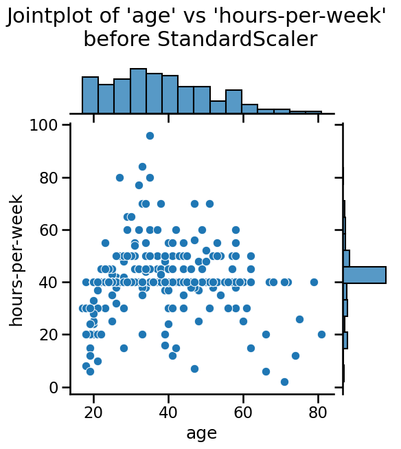
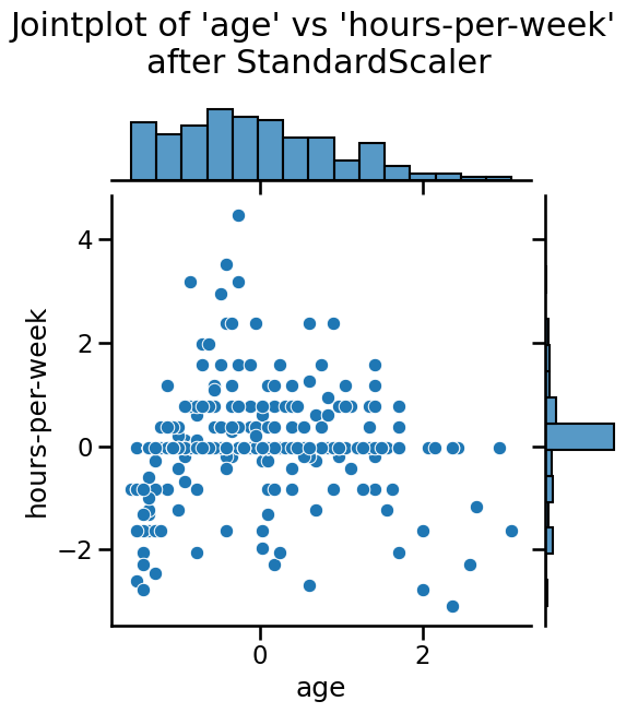
Notice that the mean of all the columns is close to 0 and the standard deviation in all cases is close to 1. We can also visualize the effect of StandardScaler using a jointplot to show both the histograms of the distributions and a scatterplot of any pair of numerical features at the same time. We can observe that StandardScaler does not change the structure of the data itself but the axes get shifted and scaled.

Note to instructor: We strongly advise to copy-paste below code and discuss the visualization with your audience. We discourage using live-coding here, because you will spend a lot of time fiddling with the jointplot, time which we can better use to introduce machine learning.

import matplotlib.pyplot as plt
import seaborn as sns

# number of points to visualize to have a clearer plot
num_points_to_plot = 300

sns.jointplot(
    data=data_train[:num_points_to_plot],
    x="age",
    y="hours-per-week",
    marginal_kws=dict(bins=15),
)
plt.suptitle(
    "Jointplot of 'age' vs 'hours-per-week' \nbefore StandardScaler", y=1.1
)

sns.jointplot(
    data=data_train_scaled[:num_points_to_plot],
    x="age",
    y="hours-per-week",
    marginal_kws=dict(bins=15),
)
_ = plt.suptitle(
    "Jointplot of 'age' vs 'hours-per-week' \nafter StandardScaler", y=1.1
)

We can easily combine sequential operations with a scikit-learn Pipeline, which chains together operations and is used as any other classifier or regressor. The helper function make_pipeline creates a Pipeline: it takes as arguments the successive transformations to perform, followed by the classifier or regressor model.

import time
from sklearn.linear_model import LogisticRegression
from sklearn.pipeline import make_pipeline

model = make_pipeline(StandardScaler(), LogisticRegression())
model

Pipeline(steps=[('standardscaler', StandardScaler()),
                ('logisticregression', LogisticRegression())])

In a Jupyter environment, please rerun this cell to show the HTML representation or trust the notebook.
On GitHub, the HTML representation is unable to render, please try loading this page with nbviewer.org.

The make_pipeline function did not require us to give a name to each step. Indeed, it was automatically assigned based on the name of the classes provided; a StandardScaler step is named "standardscaler" in the resulting pipeline. We can check the name of each steps of our model:

model.named_steps

{'standardscaler': StandardScaler(),
 'logisticregression': LogisticRegression()}

This predictive pipeline exposes the same methods as the final predictor: fit and predict (and additionally predict_proba, decision_function, or score).

model.fit(data_train, target_train)

Pipeline(steps=[('standardscaler', StandardScaler()),
                ('logisticregression', LogisticRegression())])

In a Jupyter environment, please rerun this cell to show the HTML representation or trust the notebook.
On GitHub, the HTML representation is unable to render, please try loading this page with nbviewer.org.

We can represent the internal mechanism of a pipeline when calling fit by the following diagram:

When calling model.fit, the method fit_transform from each underlying transformer (here a single transformer) in the pipeline is called to:

• learn their internal model states

• transform the training data. Finally, the preprocessed data are provided to train the predictor.

To predict the targets given a test set, one uses the predict method.

predicted_target = model.predict(data_test)
predicted_target[:5]

array([' <=50K', ' <=50K', ' >50K', ' <=50K', ' <=50K'], dtype=object)

Let’s show the underlying mechanism:

The method transform of each transformer (here a single transformer) is called to preprocess the data. Note that there is no need to call the fit method for these transformers because we are using the internal model states computed when calling model.fit. The preprocessed data is then provided to the predictor that outputs the predicted target by calling its method predict.

As a shorthand, we can check the score of the full predictive pipeline calling the method model.score. Thus, let’s check the generalization performance of such a predictive pipeline.

model_name = model.__class__.__name__
score = model.score(data_test, target_test)
print(f"The accuracy using a {model_name} is {score:.3f} ")

The accuracy using a Pipeline is 0.807 

We can compare the pipeline using scaling and logistic regression with using a logistic regression model without scaling like we did before. We will not go into how to do this comparison with Python in sake of time, instead we directly give the results:

The accuracy using a Pipeline is 0.807 with a fitting time of 0.043 seconds in 9 iterations The accuracy using a LogisticRegression is 0.807 with a fitting time of 0.110 seconds in 60 iterations

We see that scaling the data before training the logistic regression was beneficial in terms of computational performance. Indeed, the number of iterations decreased as well as the training time. The generalization performance did not change since both models converged.

Warning

Working with non-scaled data will potentially force the algorithm to iterate more as we showed in the example above. There is also the catastrophic scenario where the number of required iterations is larger than the maximum number of iterations allowed by the predictor (controlled by the max_iter) parameter. Therefore, before increasing max_iter, make sure that the data are well scaled.

Notebook recap

In scikit-learn, the score method of a classification model returns the accuracy, i.e. the fraction of correctly classified samples. In this case, around 8 / 10 of the times the logistic regression predicts the right income of a person. Now the real question is: is this generalization performance relevant of a good predictive model? Find out by solving the next exercise!

In this notebook, we learned:

• to use a scikit-learn helper to separate data into train-test sets;

• to train and evaluate a more complex scikit-learn model;

• about preprocessing for numerical variables;

• to use a scikit-learn pipeline to chain preprocessing and model training.