Vector data in Python
Last updated on 2025-02-26 | Edit this page
Overview
Questions
- How can I read, inspect, and process spatial objects, such as points, lines, and polygons?
Objectives
- Load spatial objects.
- Select the spatial objects within a bounding box.
- Perform a CRS conversion of spatial objects.
- Select features of spatial objects.
- Match objects in two datasets based on their spatial relationships.
Introduction
In the preceding episodes, we have prepared, selected and downloaded raster data from before and after the wildfire event in the summer of 2023 on the Greek island of Rhodes. To evaluate the impact of this wildfire on the vital infrastructure and built-up areas we are going to create a subset of vector data representing these assets. In this episode you will learn how to extract vector data with specific characteristics like the type of attributes or their locations. The dataset that we will generate in this episode can lateron be confronted with scorched areas which we determine by analyzing the satellite images Episode 9: Raster Calculations in Python.
We’ll be examining vector datasets that represent the valuable assests of Rhodes. As mentioned in Episode 2: Introduction to Vector Data, vector data uses points, lines, and polygons to depict specific features on the Earth’s surface. These geographic elements can have one or more attributes, like ‘name’ and ‘population’ for a city. In this episode we’ll be using two open data sources: the Database of Global Administrative Areas (GADM) dataset to generate a polygon for the island of Rhodes and and Open Street Map data for the vital infrastructure and valuable assets.
To handle the vector data in python we use the package geopandas. This
package allows us to open, manipulate, and write vector dataset through
python.
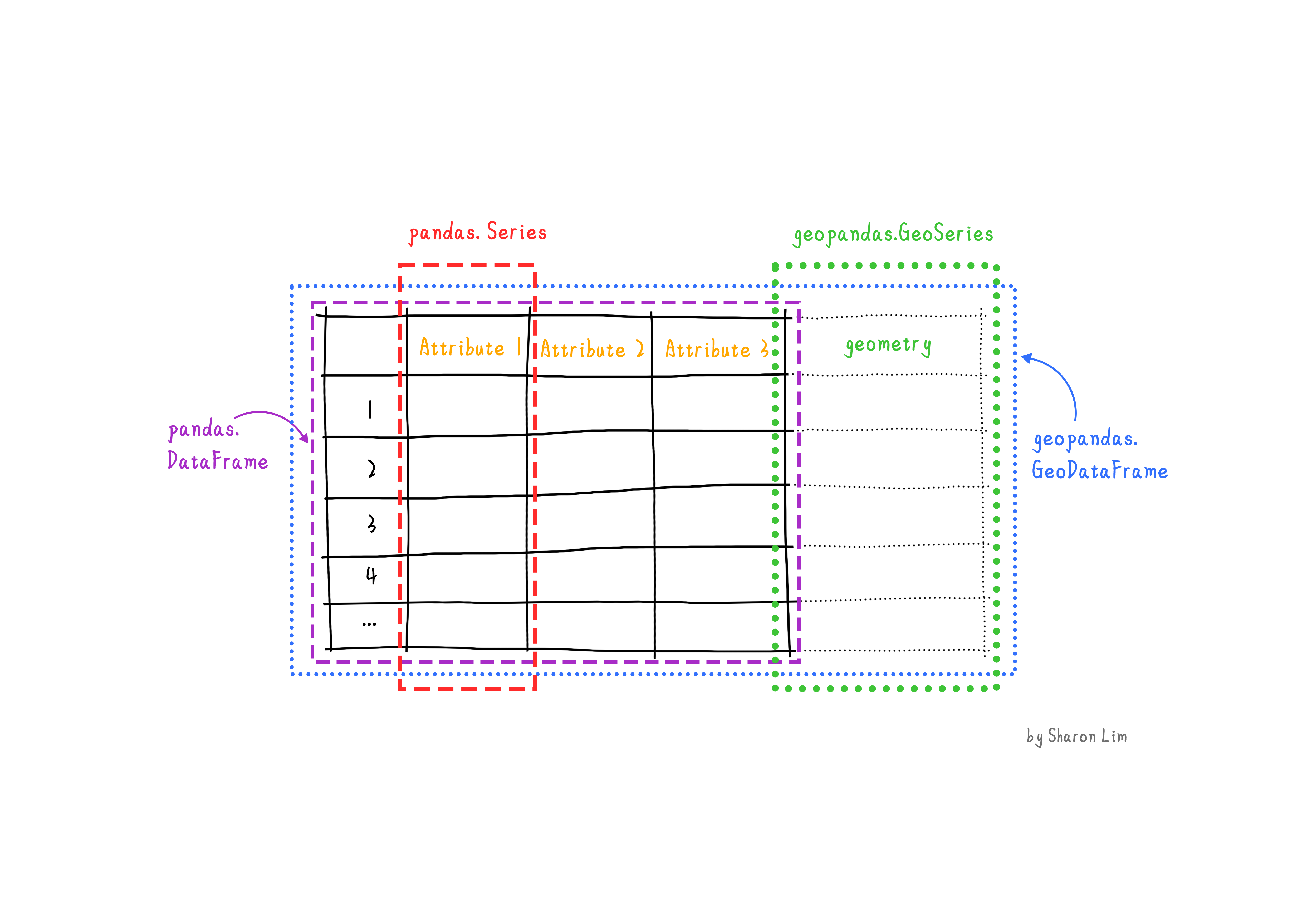
geopandas enhances the widely-used pandas
library for data analysis by extending its functionality to geospatial
applications. The primary pandas objects
(Series and DataFrame) are extended to
geopandas objects (GeoSeries and
GeoDataFrame). This extension is achieved by incorporating
geometric types, represented in Python using the shapely
library, and by offering dedicated methods for spatial operations like
union, spatial joins and
intersect. In order to understand how geopandas works, it
is good to provide a brief explanation of the relationship between
Series, a DataFrame, GeoSeries,
and a GeoDataFrame:
- A
Seriesis a one-dimensional array with an axis that can hold any data type (integers, strings, floating-point numbers, Python objects, etc.) - A
DataFrameis a two-dimensional labeled data structure with columns that can potentially hold different types of data. - A
GeoSeriesis aSeriesobject designed to store shapely geometry objects. - A
GeoDataFrameis an extendedpandas.DataFramethat includes a column with geometry objects, which is aGeoSeries.
Introduce the Vector Data
In this episode, we will use the downloaded vector data from the
data directory. Please refer to the setup page on where to download the data. Note
that we manipulated that data a little for the purposes of this
workshop. The link to the original source can be found on the setup page.
Get the administration boundary of study area
The first thing we want to do is to extract a polygon containing the
boundary of the island of Rhodes from Greece. For this we will use the
GADM dataset layer
ADM_ADM_3.gpkg for Greece. For your convenience we saved a
copy at: data/data/gadm/ADM_ADM_3.gpkg We will use the
geopandas package to load the file and use the
read_file function see.
Note that geopandas is often abbreviated as gpd.
We can print out the gdf_greecevariable:
OUTPUT
GID_3 GID_0 COUNTRY    GID_1                       NAME_1  \
0     GRC.1.1.1_1   GRC  Greece  GRC.1_1                       Aegean
1     GRC.1.1.2_1   GRC  Greece  GRC.1_1                       Aegean
2     GRC.1.1.3_1   GRC  Greece  GRC.1_1                       Aegean
..            ...   ...     ...      ...                          ...
324  GRC.8.2.24_1   GRC  Greece  GRC.8_1  Thessaly and Central Greece
325  GRC.8.2.25_1   GRC  Greece  GRC.8_1  Thessaly and Central Greece

                      NL_NAME_1      GID_2        NAME_2      NL_NAME_2  \
0                        Αιγαίο  GRC.1.1_1  North Aegean  Βόρειο Αιγαίο
1                        Αιγαίο  GRC.1.1_1  North Aegean  Βόρειο Αιγαίο
2                        Αιγαίο  GRC.1.1_1  North Aegean  Βόρειο Αιγαίο
..                          ...        ...           ...            ...
324  Θεσσαλία και Στερεά Ελλάδα  GRC.8.2_1      Thessaly       Θεσσαλία
325  Θεσσαλία και Στερεά Ελλάδα  GRC.8.2_1      Thessaly       Θεσσαλία
...
324  POLYGON ((22.81903 39.27344, 22.81884 39.27332...
325  POLYGON ((23.21375 39.36514, 23.21272 39.36469...

[326 rows x 17 columns]
The data are read into the variable fields as a
GeoDataFrame. This is an extened data format of
pandas.DataFrame, with an extra column
geometry. To explore the dataframe you can call this
variable just like a pandas dataframe by using functions
like .shape, .head and .tail
etc.
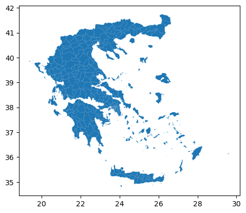
To visualize the polygons we can use the plot()
function to the GeoDataFrame we have loaded
gdf_greece:
If you want to interactively explore your data you can use the .explore
function in geopandas:
In this interactive map you can easily zoom in and out and hover over the polygons to see which attributes, stored in the rows of your GeoDataFrame, are related to each polygon.
Next, we’ll focus on isolating the administrative area of Rhodes
Island. Once you hover over the polygon of Rhodos (the relatively big
island to the east) you will find out that the label Rhodos
is stored in the NAME_3 column of gdf_greece,
where Rhodes Island is listed as Rhodos. Since our goal is
to have a boundary of Rhodes, we’ll now create a new variable that
exclusively represents Rhodes Island.
To select an item in our GeoDataFrame with a specific value is done
the same way in which this is done in a pandas DataFrame
using .loc.
And we can plot the overview by (or show it interactively using
.explore):
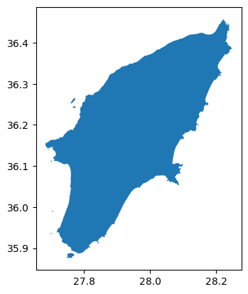
Now that we have the administrative area of Rhodes Island. We can use
the to_file() function save this file for future use.
Get the vital infrastructure and built-up areas
Road data from Open Street Map (OSM)
Now that we have the boundary of our study area, we will make use this to select the main roads in our study area. We will make the following processing steps:
- Select roads of study area
- Select key infrastruture: ‘primary’, ‘secondary’, ‘tertiary’
- Create a 100m buffer around the rounds. This buffer will be regarded as the infrastructure region. (note that this buffer is arbitrary and can be changed afterwards if you want!)
Step 1: Select roads of study area
For this workshop, in particular to not have everyone downloading too
much data, we created a subset of the Openstreetmap data we
downloaded for Greece from the Geofabrik. This
data comes in the form of a shapefile (see episode 2) from which we extracted
all the roads for Rhodes and some surrounding islands. The
data is stored in the osm folder as osm_roads.gpkg, but
contains all the roads on the island (so also hiking paths,
private roads etc.), whereas we in particular are interested in the key
infrastructure which we consider to be roads classified as primary,
secondary or tertiary roads.
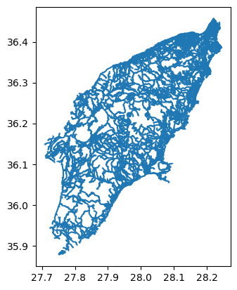
Let’s load the file and plot it:
We can explore it using the same commands as above:
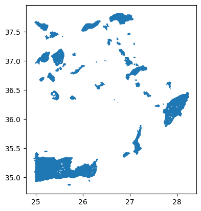
As you may have noticed, loading and plotting
osm_roads.gpkg takes a bit long. This is because the file
contains all the roads of Rhodos and some surrounding islands as well.
Since we are only interested in the roads on Rhodes Island. We will use
the mask
parameter of the read_file() function to load only the
roads on Rhodes Island.
Now let us overwrite the GeoDataframe gdf_roads using
the mask with the GeoDataFrame gdf_rhodes we created
above.
Now let us explore these roads using .explore (or
.plot):
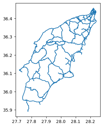
Step 2: Select key infrastruture
As you will find out while exploring the roads dataset, information
about the type of roads is stored in the fclass column. To
get an overview of the different values that are present in the collumn
fclass , we can use the unique()
function from pandas:
OUTPUT
array(['residential', 'service', 'unclassified', 'footway',
       'track_grade4', 'primary', 'track', 'tertiary', 'track_grade3',
       'path', 'track_grade5', 'steps', 'secondary', 'primary_link',
       'track_grade2', 'track_grade1', 'pedestrian', 'tertiary_link',
       'secondary_link', 'living_street', 'cycleway'], dtype=object)
It seems the variable gdf_roads contains all kind of
hiking paths and footpaths as well. Since we are only interested in
vital infrastructure, classified as “primary”, “secondary” and
“tertiary” roads, we need to make a subselection.
Let us first create a list with the labels we want to select.
Now we are using this list make a subselection of the key
infrastructure using pandas´ .isin
function.
We can plot the key infrastructure :
Step 3: Create a 100m buffer around the key infrastructure
Now that we selected the key infrastructure, we want to create a 100m buffer around them. This buffer will be regarded as the infrastructure region.
As you might have notice, the numbers on the x and y axis of our plots represent Lon Lat coordinates, meaning that the data is not yet projected. The current data has a geographic coordinate system with measures in degrees but not meter. Creating a buffer of 100 meters is not possible. Therfore, in order to create a 100m buffer, we first need to project our data. In our case we decided to project the data as WGS 84 / UTM zone 31N, with EPSG code 32631 (see chapter 03 for more information about the CRS and EPSG codes.
To project our data we use .to_crs. We first define a variable with the EPSG value (in our case 32631), which we then us in the to_crs function.
Now that our data is projected, we can create a buffer. For this we make use of geopandas´ .buffer function :
OUTPUT
53       POLYGON ((2779295.383 4319805.295, 2779317.029...
54       POLYGON ((2779270.962 4319974.441, 2779272.393...
55       POLYGON ((2779172.341 4319578.062, 2779165.312...
84       POLYGON ((2779615.109 4319862.058, 2779665.519...
140      POLYGON ((2781330.698 4320046.538, 2781330.749...
                               ...
19020    POLYGON ((2780193.230 4337691.133, 2780184.279...
19021    POLYGON ((2780330.823 4337772.262, 2780324.966...
19022    POLYGON ((2780179.850 4337917.135, 2780188.871...
19024    POLYGON ((2780516.550 4339028.863, 2780519.340...
19032    POLYGON ((2780272.050 4338213.937, 2780274.519...
Length: 1386, dtype: geometry
Note that the type of the key_infra_meters_buffer is a
GeoSeries and not a GeoDataFrame. This is
because the buffer() function returns a
GeoSeries object. You can check that by calling the type of
the variable.
OUTPUT
geopandas.geoseries.GeoSeriesNow that we have a buffer, we can convert it back to the geographic
coordinate system to keep the data consistent. Note that we are now
using the crs information from the key_infra, instead of
using the EPSG code directly (EPSG:4326):
OUTPUT
45       POLYGON ((27.72826 36.12409, 27.72839 36.12426...
58       POLYGON ((27.71666 36.11678, 27.71665 36.11678...
99       POLYGON ((27.75485 35.95242, 27.75493 35.95248...
100      POLYGON ((27.76737 35.95086, 27.76733 35.95086...
108      POLYGON ((27.76706 35.95199, 27.76702 35.95201...
                               ...
18876    POLYGON ((28.22855 36.41890, 28.22861 36.41899...
18877    POLYGON ((28.22819 36.41838, 28.22825 36.41845...
18878    POLYGON ((28.22865 36.41904, 28.22871 36.41912...
18879    POLYGON ((28.23026 36.41927, 28.23034 36.41921...
18880    POLYGON ((28.23020 36.41779, 28.23007 36.41745...
Length: 1369, dtype: geometry
As you can see, the buffers created in key_infra_buffer
have the Polygon geometry type.
To double check the EPSG code of key_infra:
OUTPUT
EPSG:4326Reprojecting and buffering our data is something that we are going to do multiple times during this episode. To avoid have to call the same functions multiple times it would make sense to create a function. Therefore, let us create a function in which we can add the buffer as a variable.
PYTHON
def buffer_crs(gdf, size, meter_crs=32631, target_crs=4326):
    return gdf.to_crs(meter_crs).buffer(size).to_crs(target_crs)
For example, we can use this function to create a 200m buffer around the infrastructure the key infrastructure by doing:
Get built-up regions from Open Street Map (OSM)
Now that we have a buffered dataset for the key infrastructure of
Rhodes, our next step is to create a dataset with all the built-up
areas. To do so we will use the land use data from OSM, which we
prepared for you in the file data/osm_landuse.gpkg. This
file includes the land use data for the entire Greece. We assume the
built-up regions to be the union of three types of land use:
“commercial”, “industrial”, and “residential”.
Note that for the simplicity of this course, we limit the built-up regions to these three types of land use. In reality, the built-up regions can be more complex also there is definately more high quality (e.g. local government).
Now it will be up to you to create a dataset with valueable assets. You should be able to complete this task by yourself with the knowledge you have gained from the previous steps and links to the documentation we provided.
Exercise: Get the built-up regions
Create a builtup_buffer from the file
data/osm/osm_landuse.gpkg by the following steps:
- Load the land use data from
data/osm/osm_landuse.gpkgand mask it with the administrative boundary of Rhodes Island (gdf_rhodes). - Select the land use data for “commercial”, “industrial”, and “residential”.
- Create a 10m buffer around the land use data.
- Visualize the results.
After completing the exercise, answer the following questions:
- How many unique land use types are there in
osm_landuse.gpkg? - After selecting the three types of land use, how many entries (rows) are there in the results?
Hints:
-
data/osm_landuse.gpkgcontains the land use data for the entire Greece. Use the administrative boundary of Rhodes Island (gdf_rhodes) to select the land use data for Rhodes Island. - The land use attribute is stored in the
fclasscolumn. - Reuse
buffer_crsfunction to create the buffer.
PYTHON
# Read data with a mask of Rhodes
gdf_landuse = gpd.read_file('./data/osm/osm_landuse.gpkg', mask=gdf_rhodes)

# Find number of unique landuse types
print(len(gdf_landuse['fclass'].unique()))

# Extract built-up regions
builtup_labels = ['commercial', 'industrial', 'residential']
builtup = gdf_landuse[gdf_landuse['fclass'].isin(builtup_labels)]

# Create 10m buffer around the built-up regions
builtup_buffer = buffer_crs(builtup, 10)

# Get the number of entries
print(len(builtup_buffer))

# Visualize the buffer
builtup_buffer.plot()
OUTPUT
19
1349
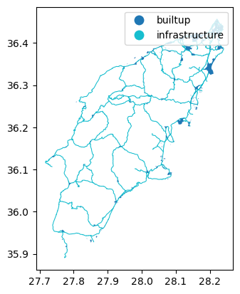
Merge the infrastructure regions and built-up regions
Now that we have the infrastructure regions and built-up regions, we
can merge them into a single region. We would like to keep track of the
type after merging, so we will add two new columns: type
and code by converting the GeoSeries to
GeoDataFrame.
First we convert the buffer around key infrastructure:
PYTHON
data = {'geometry': key_infra_buffer, 'type': 'infrastructure', 'code': 1}
gdf_infra = gpd.GeoDataFrame(data)
Then we convert the built-up buffer:
PYTHON
data = {'geometry': builtup_buffer, 'type': 'builtup', 'code': 2}
gdf_builtup = gpd.GeoDataFrame(data)
After that, we can merge the two GeoDataFrame into
one:
In gdf_assets, we can distinguish the infrastructure
regions and built-up regions by the type and
code columns. We can plot the gdf_assets to
visualize the merged regions. See the geopandas
documentation on how to do this:
Finally, we can save the gdf_assets to a file for future
use:
- Load spatial objects into Python with
geopandas.read_file()function. - Spatial objects can be plotted directly with
GeoDataFrame’s.plot()method. - Convert CRS of spatial objects with
.to_crs(). Note that this generates aGeoSeriesobject. - Create a buffer of spatial objects with
.buffer(). - Merge spatial objects with
pd.concat().