Calculating Zonal Statistics on Rasters

Estimated time: 40 minutes

Overview

Questions

• How to compute raster statistics on different zones delineated by vector data?

Objectives

• Extract zones from the vector dataset
• Convert vector data to raster
• Calculate raster statistics over zones

Introduction

---

Statistics on predefined zones of the raster data are commonly used for analysis and to better understand the data. These zones are often provided within a single vector dataset, identified by certain vector attributes. For example, in the previous episodes, we defined infrastructure regions and built-up regions on Rhodes Island as polygons. Each region can be respectively identified as a “zone”, resulting in two zones. One can evualuate the effect of the wild fire on the two zones by calculating the zonal statistics.

Data loading

---

We have created assets.gpkg in Episode “Vector data in Python”, which contains the infrastructure regions and built-up regions . We also calculated the burned index in Episode “Raster Calculations in Python” and saved it in burned.tif. Lets load them:

PYTHON

# Load burned index
import rioxarray
burned = rioxarray.open_rasterio('burned.tif')

# Load assests polygons
import geopandas as gpd
assets = gpd.read_file('assets.gpkg')

Align datasets

---

Before we continue, let’s check if the two datasets are in the same CRS:

PYTHON

print(assets.crs)
print(burned.rio.crs)

OUTPUT

EPSG:4326
EPSG:32635

The two datasets are in different CRS. Let’s reproject the assets to the same CRS as the burned index raster:

PYTHON

assets = assets.to_crs(burned.rio.crs)

Rasterize the vector data

---

One way to define the zones, is to create a grid space with the same extent and resolution as the burned index raster, and with the numerical values in the grid representing the type of infrastructure, i.e., the zones. This can be done by rasterize the vector data assets to the grid space of burned.

Let’s first take two elements from assets, the geometry column, and the code of the region.

PYTHON

geom = assets[['geometry', 'code']].values.tolist()
geom

OUTPUT

[[<POLYGON ((569708.927 3972332.358, 569709.096 3972333.79, 569710.406 3972341...>,
  1],
 [<MULTIPOLYGON (((567767.095 3970740.732, 567767.548 3970741.604, 567772.083 ...>,
  2]]

The raster image burned is a 3D image with a “band” dimension.

PYTHON

burned.shape

OUTPUT

(1, 1131, 1207)

To create the grid space, we only need the two spatial dimensions. We can used .squeeze() to drop the band dimension:

PYTHON

burned_squeeze = burned.squeeze()
burned_squeeze.shape

OUTPUT

(1131, 1207)

Now we can use features.rasterize from rasterio to rasterize the vector data assets to the grid space of burned:

PYTHON

from rasterio import features
assets_rasterized = features.rasterize(geom, out_shape=burned_squeeze.shape, transform=burned.rio.transform())
assets_rasterized

OUTPUT

array([[0, 0, 0, ..., 0, 0, 0],
       [0, 0, 0, ..., 0, 0, 0],
       [0, 0, 0, ..., 0, 0, 0],
       ...,
       [0, 0, 0, ..., 0, 0, 0],
       [0, 0, 0, ..., 0, 0, 0],
       [0, 0, 0, ..., 0, 0, 0]], dtype=uint8)

Perform zonal statistics

---

The rasterized zones assets_rasterized is a numpy array. The Python package xrspatial, which is the one we will use for zoning statistics, accepts xarray.DataArray. We need to first convert assets_rasterized. We can use burned_squeeze as a template:

PYTHON

assets_rasterized_xarr = burned_squeeze.copy()
assets_rasterized_xarr.data = assets_rasterized
assets_rasterized_xarr.plot()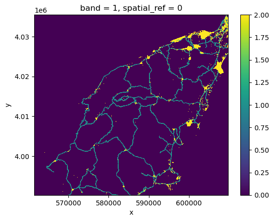

Then we can calculate the zonal statistics using the zonal_stats function:

PYTHON

from xrspatial import zonal_stats
stats = zonal_stats(assets_rasterized_xarr, burned_squeeze)
stats

OUTPUT

    zone	  mean	    max	min	sum	    std	      var	      count
0	    0	    0.022570	1.0	0.0	28929.0	0.148528	0.022061	1281749.0
1	    1	    0.009607	1.0	0.0	568.0	  0.097542	0.009514	59125.0
2	    2	    0.000000	0.0	0.0	0.0	    0.000000	0.000000	24243.0

The results provide statistics for three zones: 1 represents infrastructure regions, 2 represents built-up regions, and 0 represents the rest of the area.

Key Points

• Zones can be extracted by attribute columns of a vector dataset
• Zones can be rasterized using rasterio.features.rasterize
• Calculate zonal statistics with xrspatial.zonal_stats over the rasterized zones.