All Images
Introduction to Raster Data
Figure 1
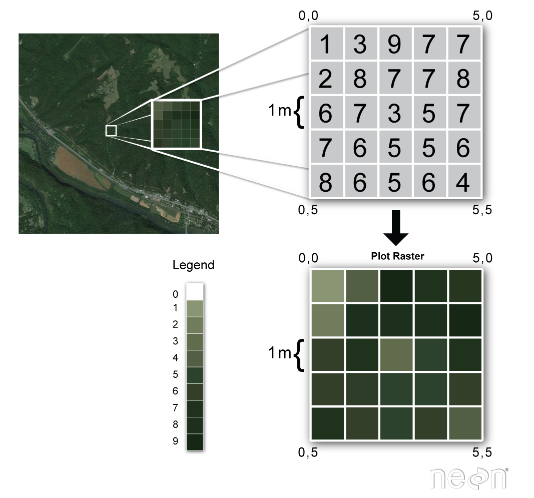
Raster Concept (Source: National Ecological
Observatory Network (NEON))
Figure 2
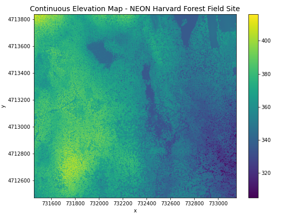
Continuous Elevation Map: HARV Field Site
Figure 3
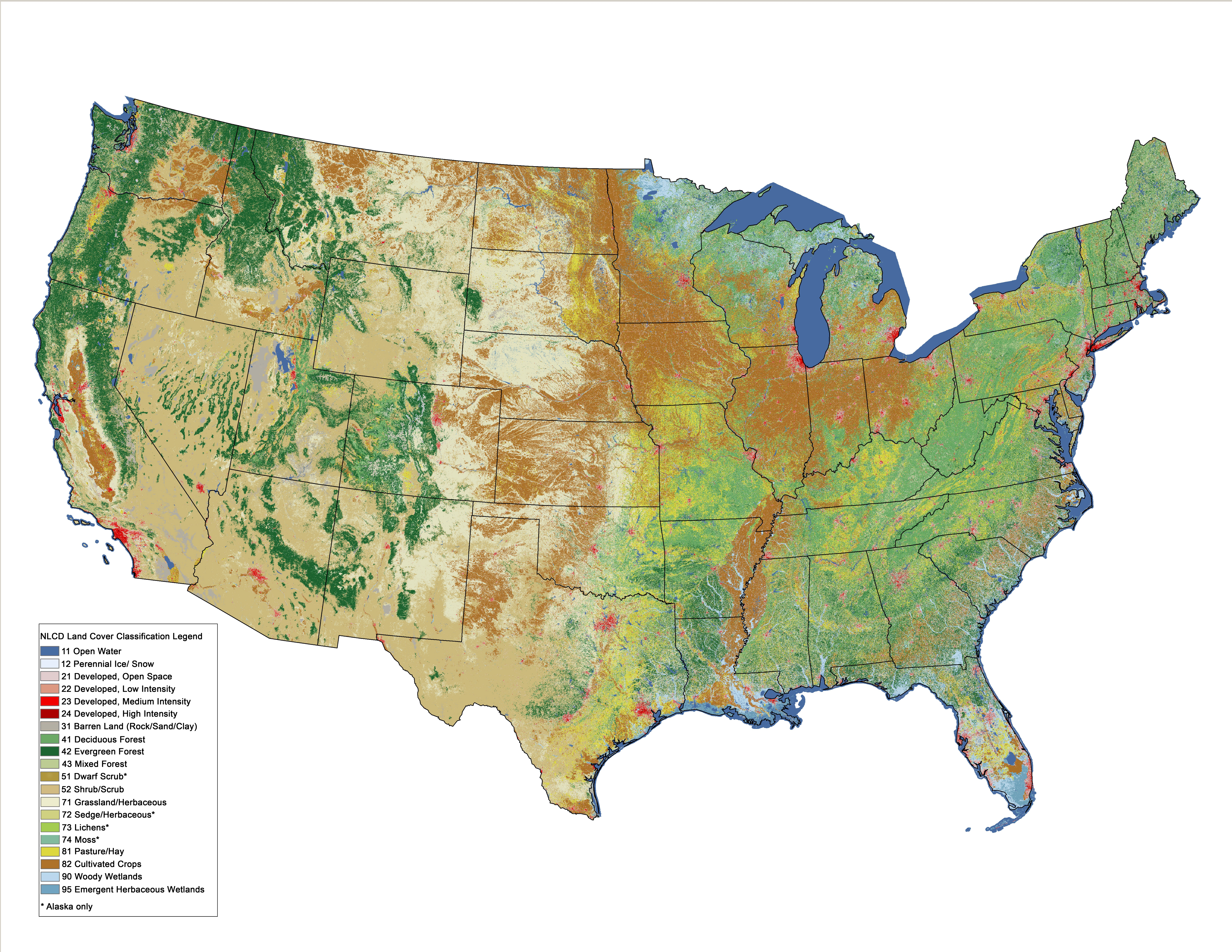
USA landcover classification
Figure 4
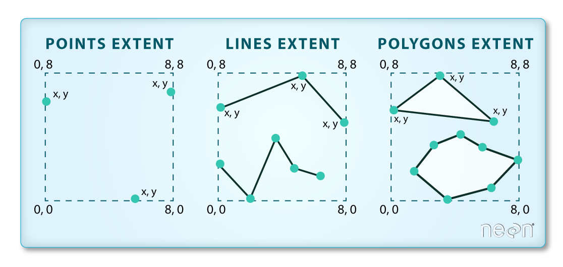
Spatial extent image (Image Source: National
Ecological Observatory Network (NEON))
Figure 5
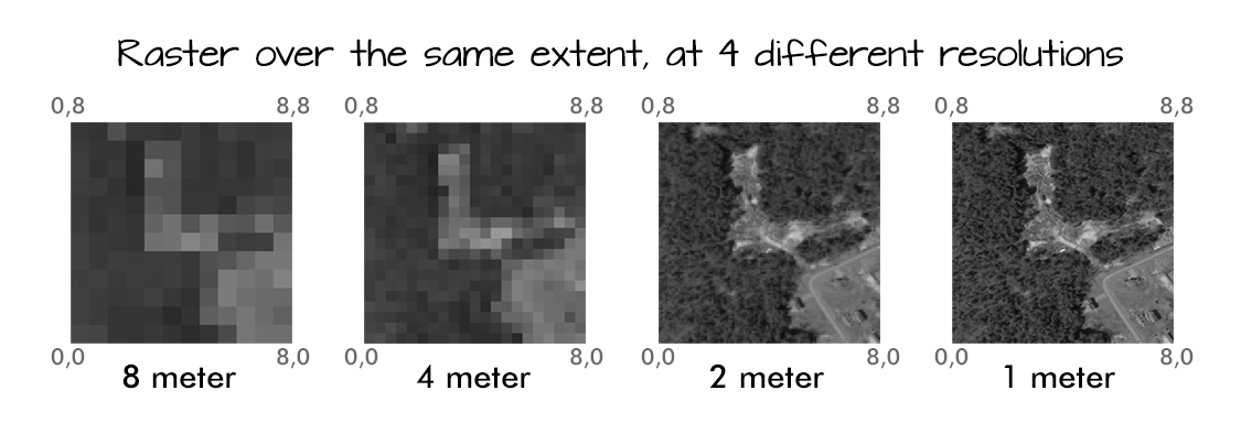
Resolution image (Source: National Ecological
Observatory Network (NEON))
Figure 6
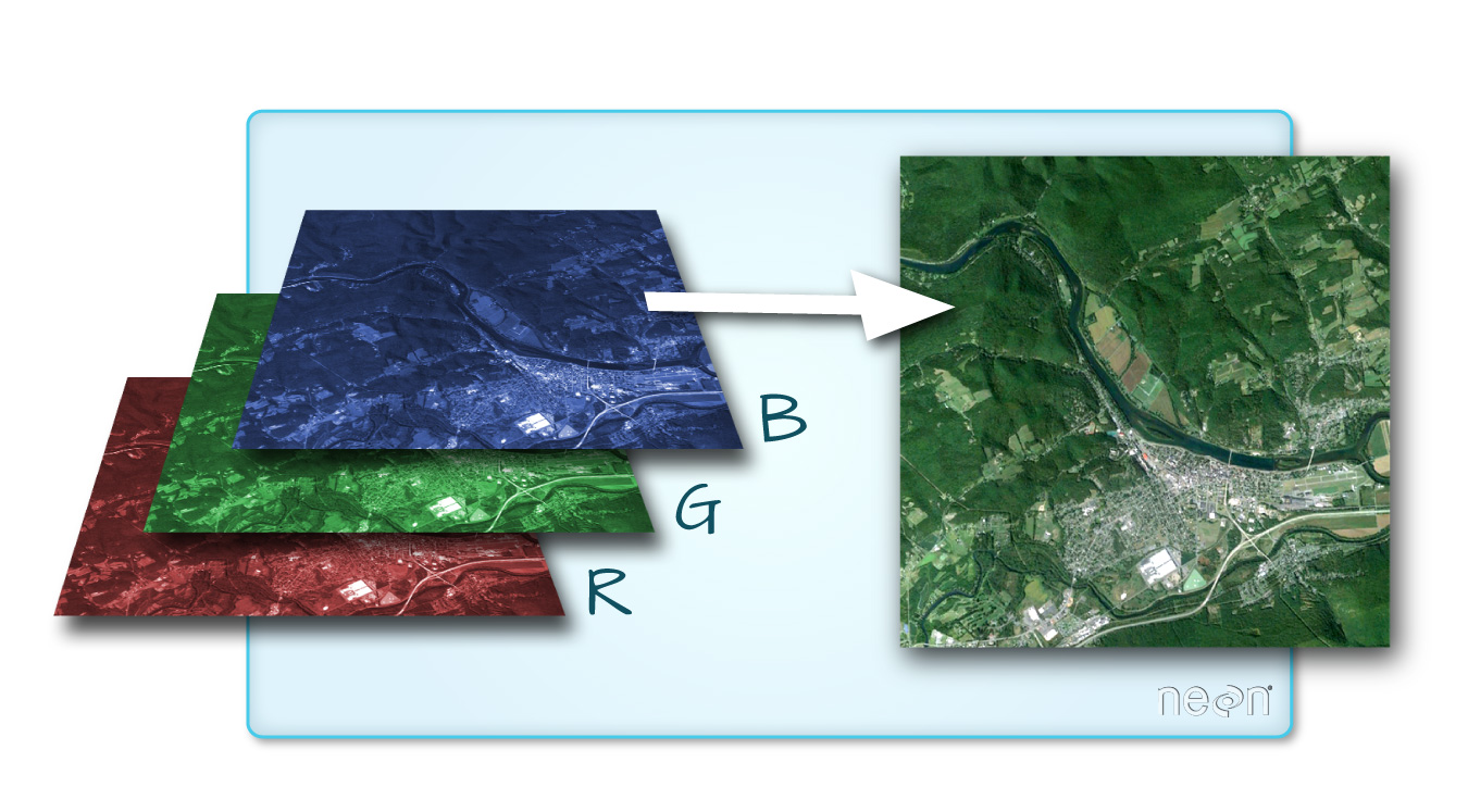
RGB multi-band raster image (Source: National
Ecological Observatory Network (NEON).)
Introduction to Vector Data
Figure 1
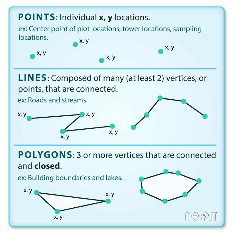
Types of vector objects (Image Source: National
Ecological Observatory Network (NEON))
Figure 2
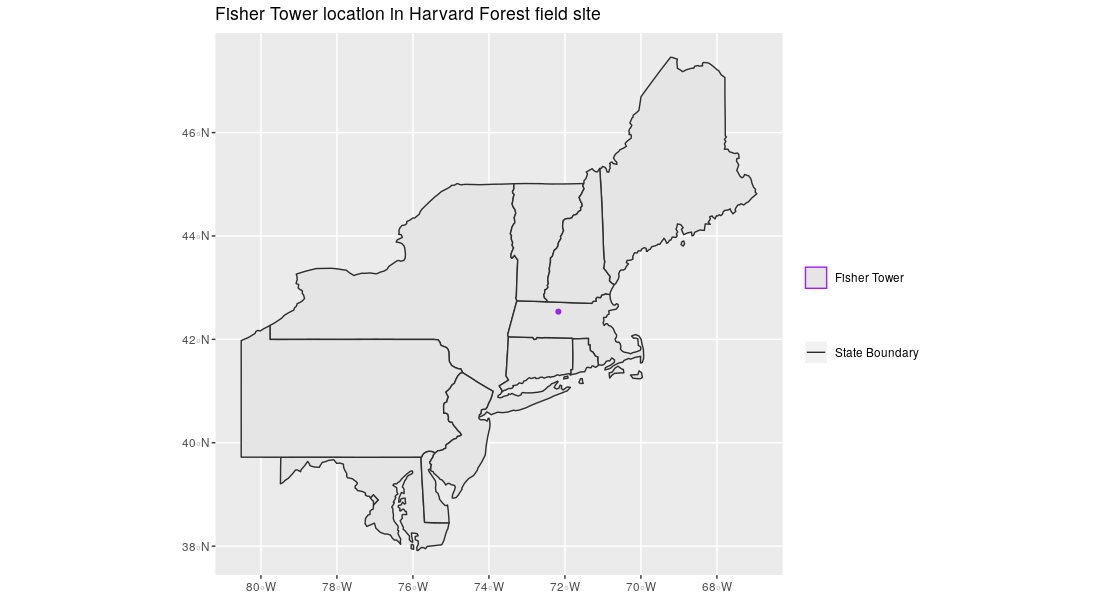
Vector Type Examples
Coordinate Reference Systems
Figure 1
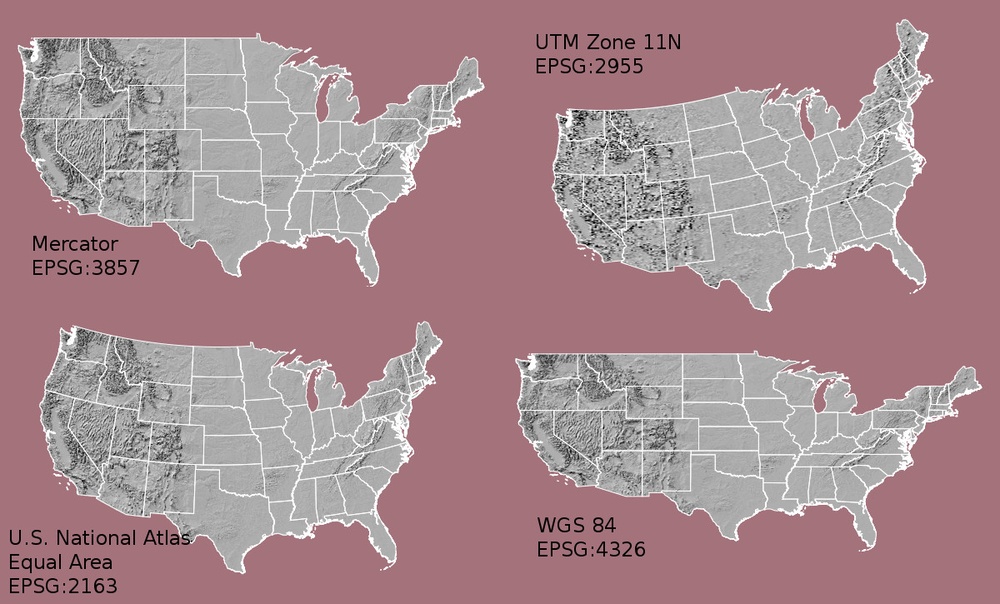
Figure 3.1: Maps of the United States in
different projections (Source: opennews.org)
Figure 2
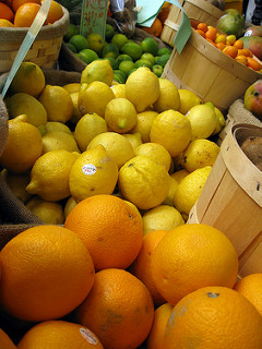
Datum Fruit Example (Image
source)
Figure 3
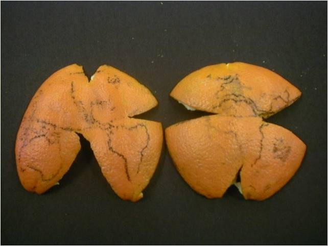
Projection Citrus Peel Example (Image from Prof
Drika Geografia, Projeções Cartográficas)
Figure 4

The UTM zones across the continental United
States (Chrismurf at English Wikipedia, via Wikimedia
Commons (CC-BY))
The Geospatial Landscape
Access satellite imagery using Python
Figure 1
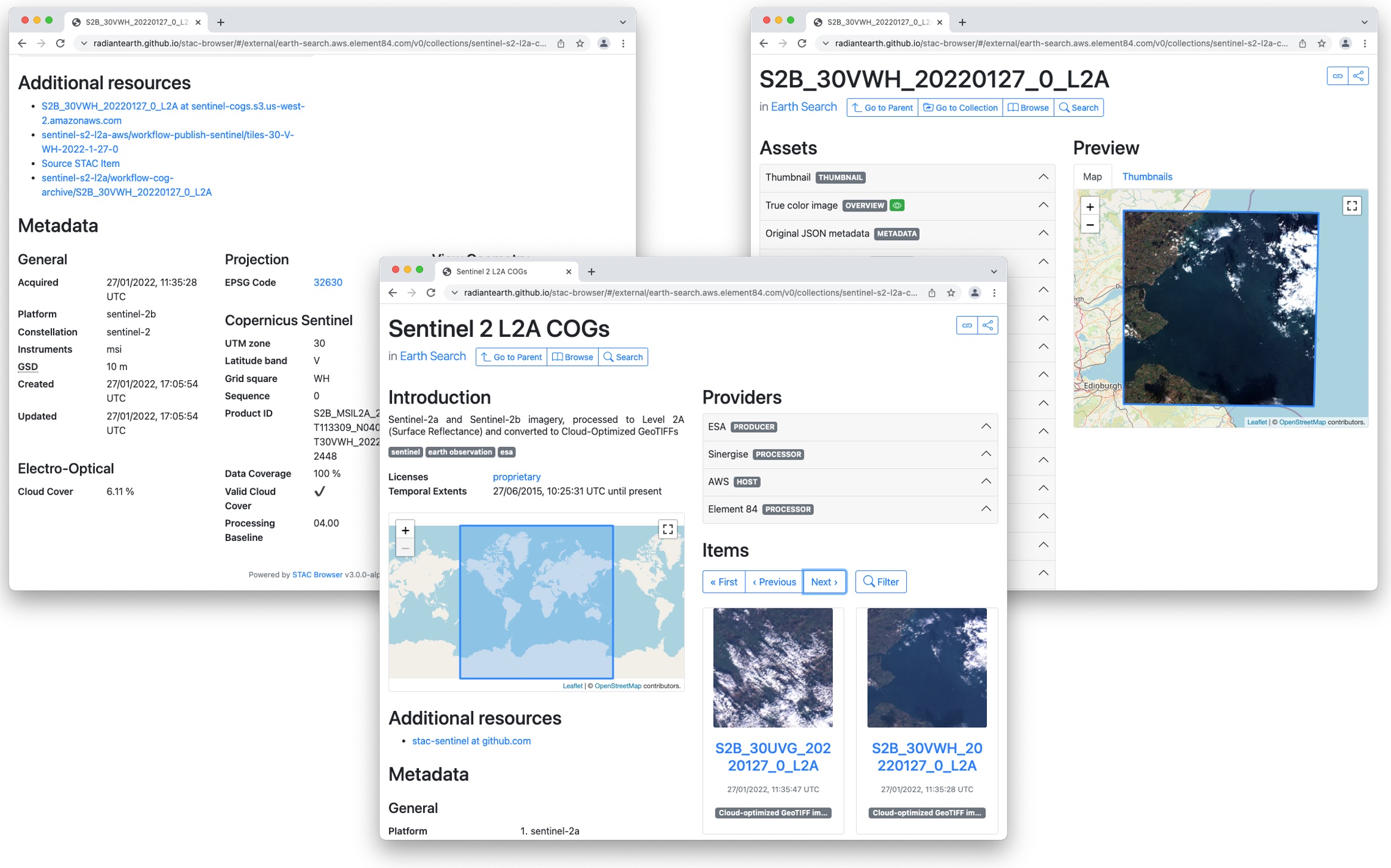
Views of the STAC browser
Figure 2
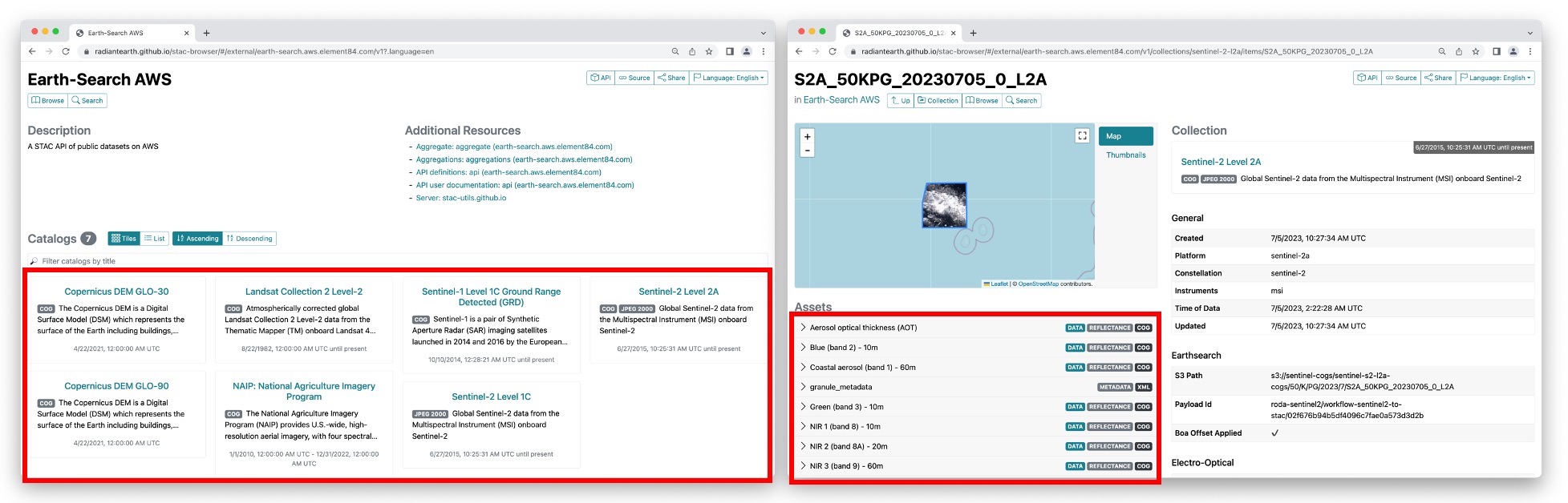
Views of the Earth Search STAC endpoint
Figure 3
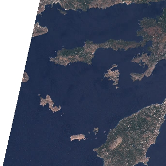
Overview of the true-color image (“thumbnail”)
before the wildfires on Rhodes
Figure 4
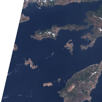
Overview of the true-color image (“thumbnail”)
after the wildfires on Rhodes
Figure 5
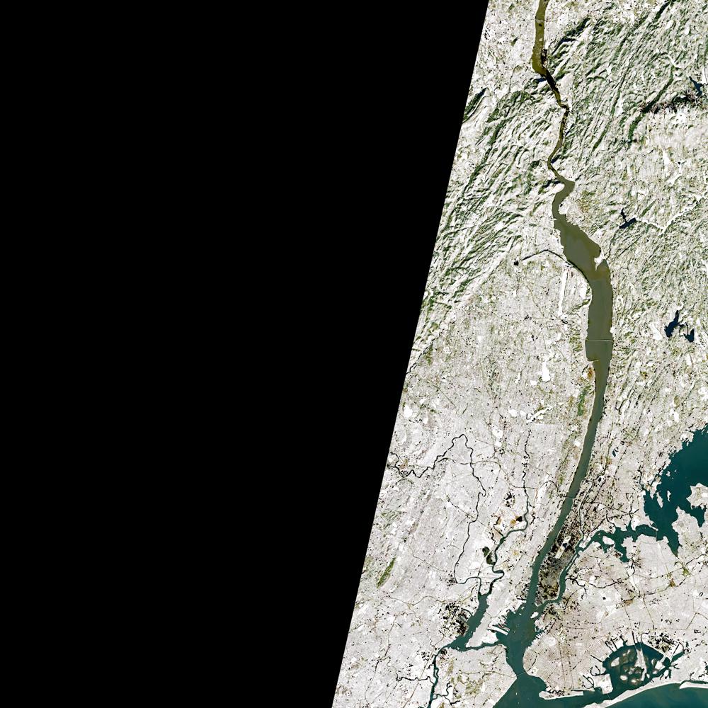
Thumbnail of the Landsat-8 scene
Read and visualize raster dataResampling the raster image
Figure 1
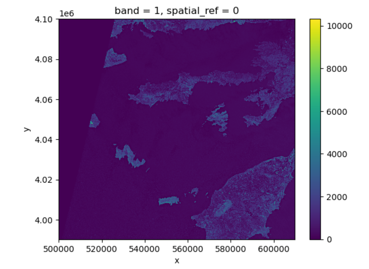
Raster plot with rioxarray
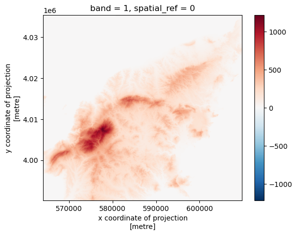
Figure 2
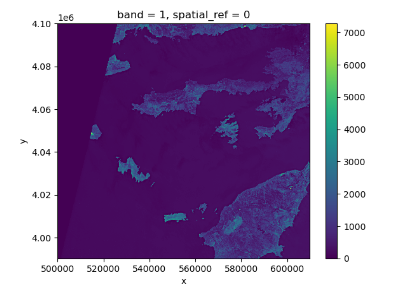
Raster plot 80 x 80 meter resolution with
rioxarray
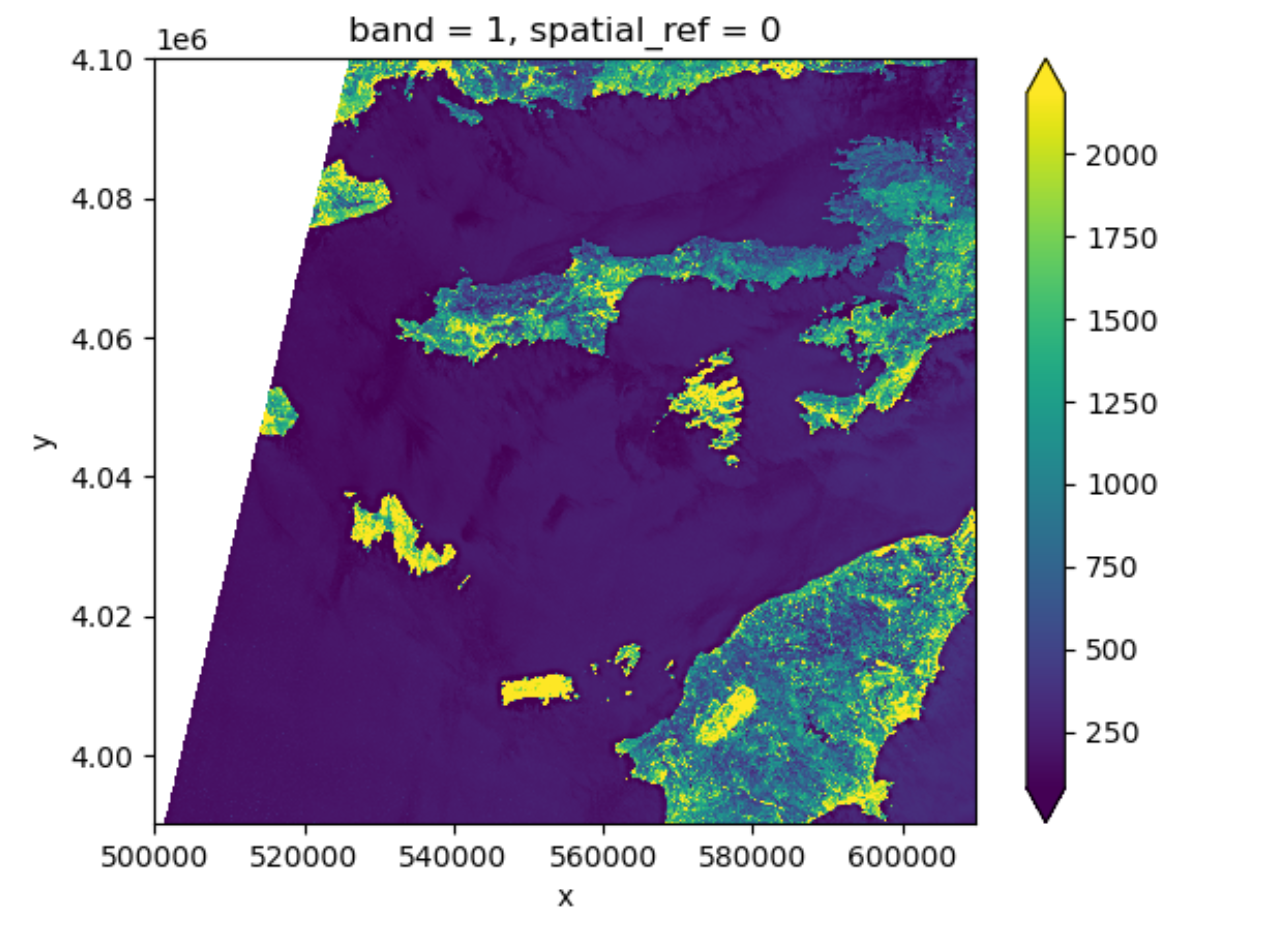
Figure 3
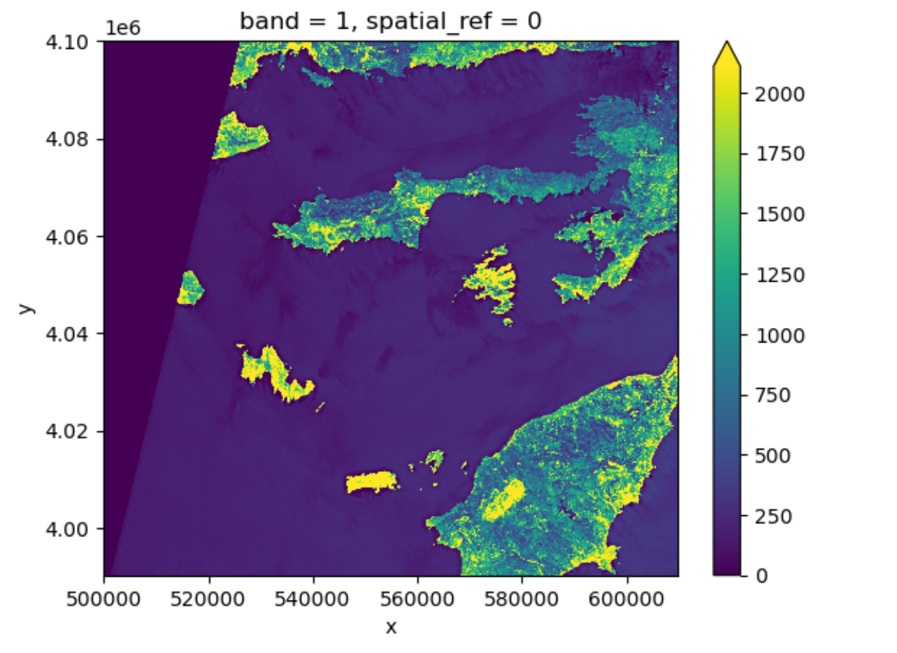
Raster plot using the “robust” setting
Figure 4
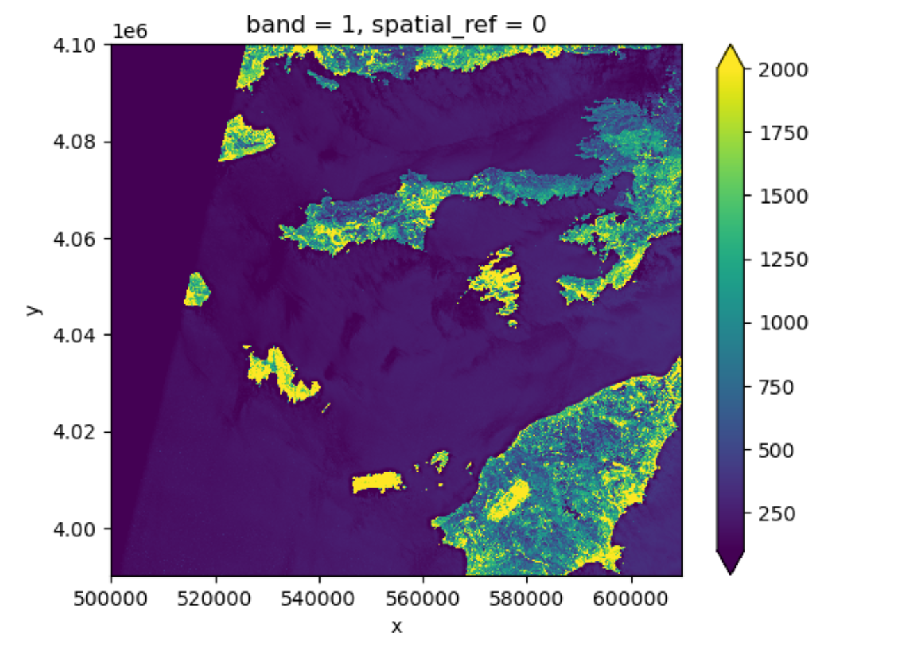
Raster plot using vmin 100 and vmax 2000
Figure 5
The UTM zones across the continental United
States (Chrismurf at English Wikipedia, via Wikimedia
Commons (CC-BY))
Figure 6
Raster plot after masking out missing
values
Figure 7
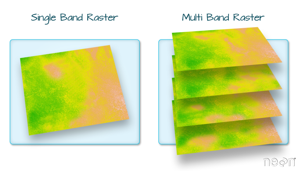
Sketch of a multi-band raster image
Figure 8
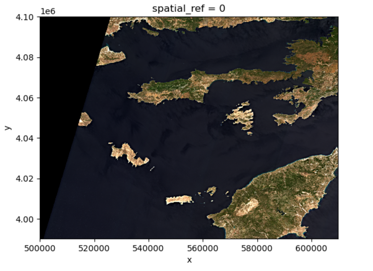
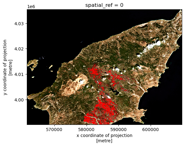
Overview of the true-color image (multi-band
raster)
Figure 9
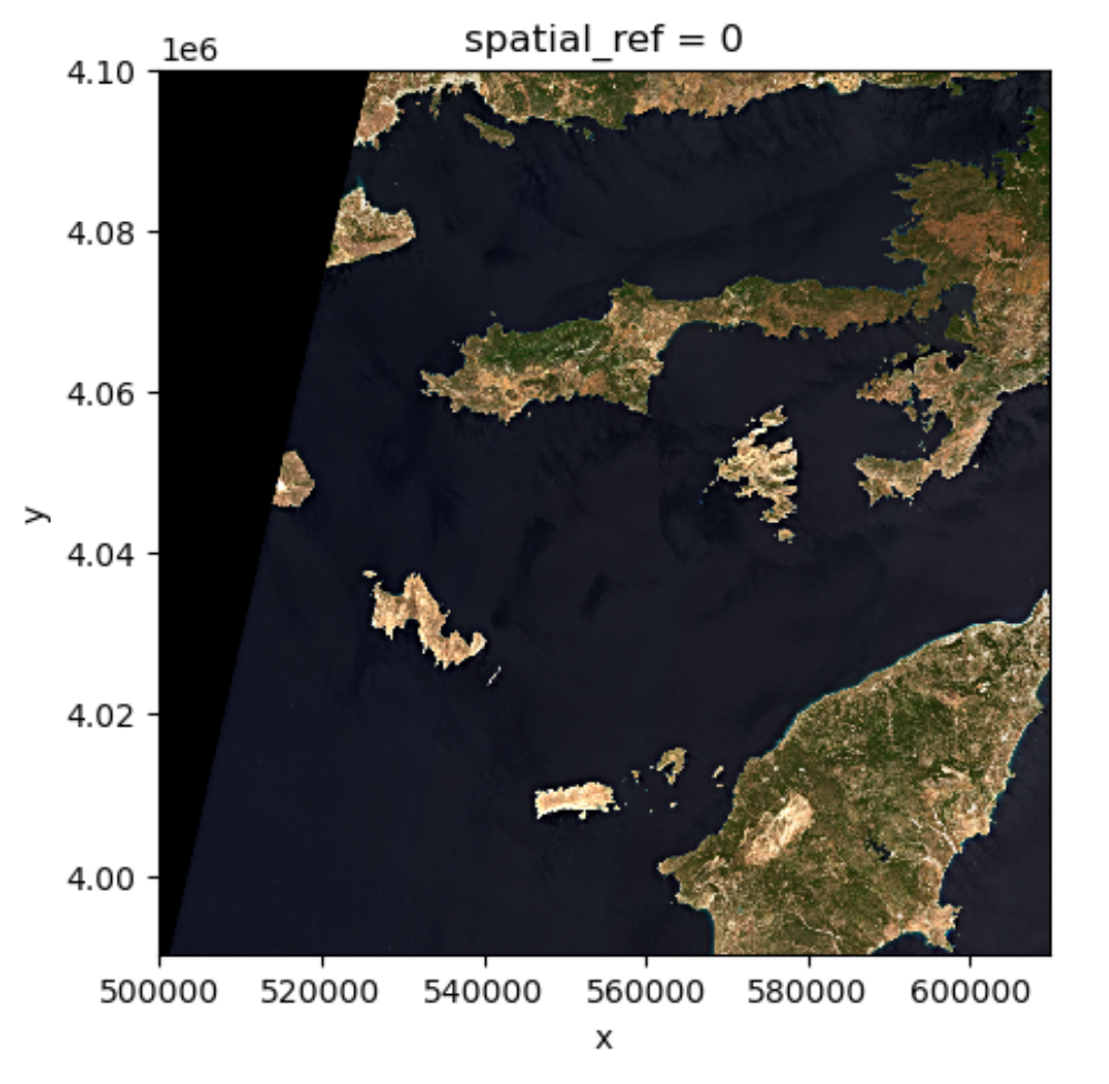
Overview of the true-color image with the
correct aspect ratio
Vector data in Python
Figure 1
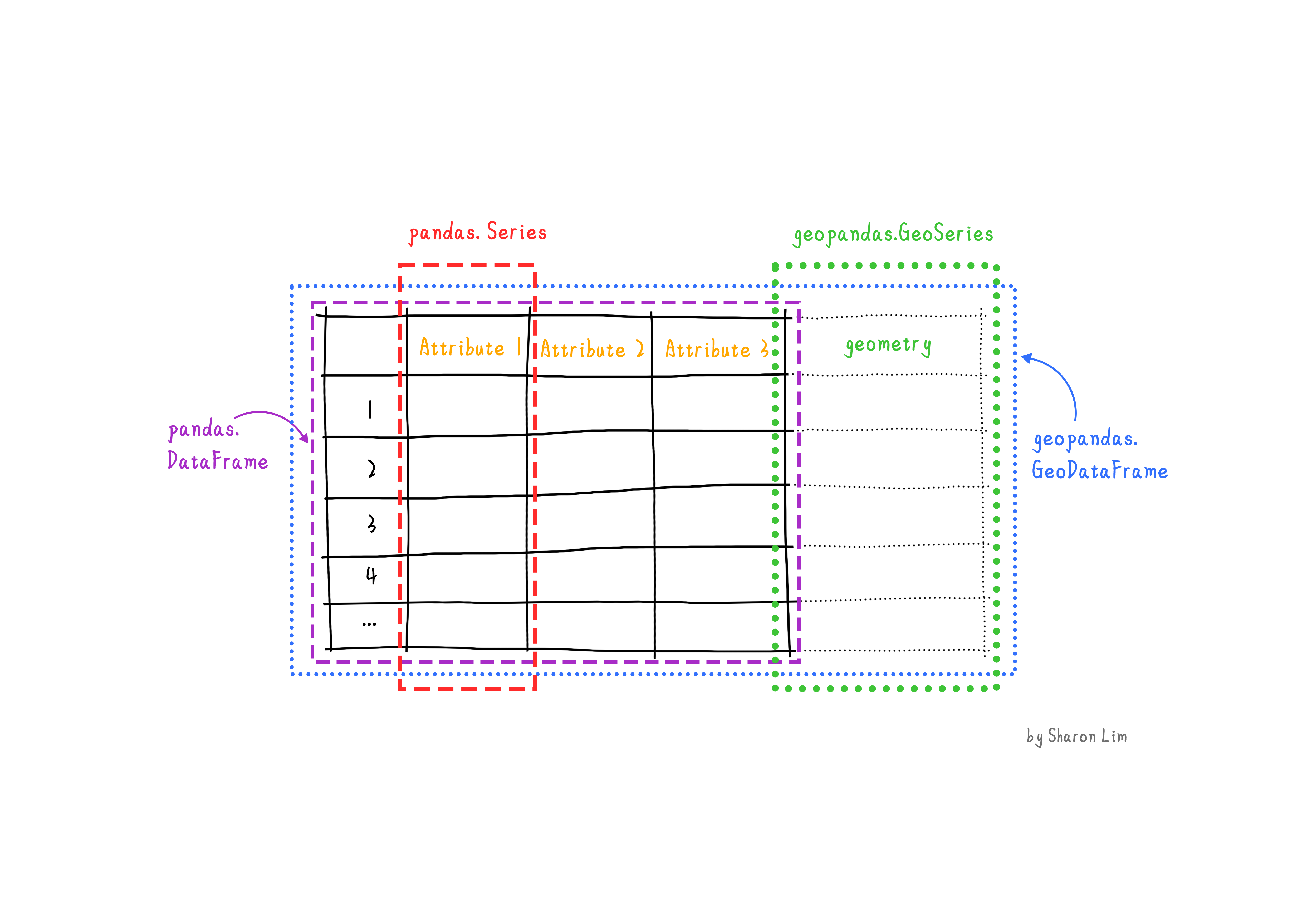
Figure 2
Figure 3
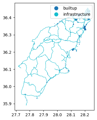
Figure 4
Figure 5
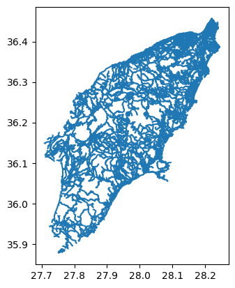
Figure 6
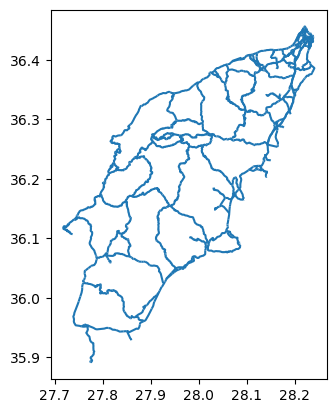
Figure 7
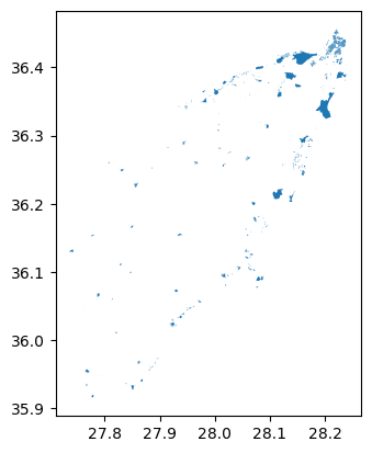
Figure 8
Crop raster data with rioxarray and geopandas
Figure 1
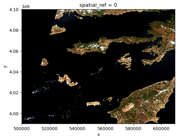
Figure 2
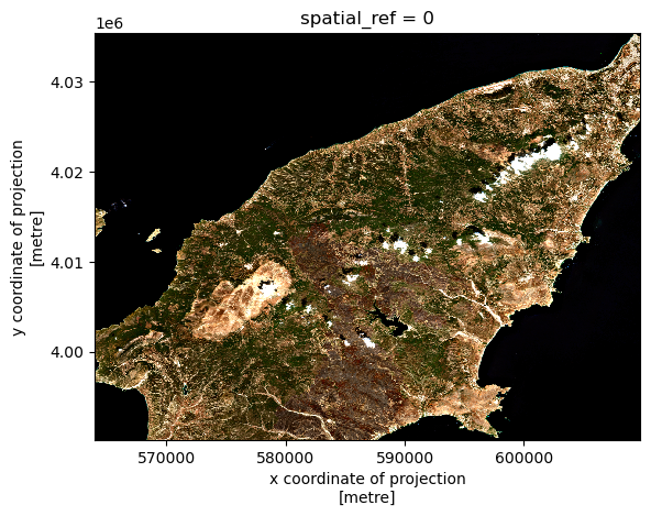
Figure 3
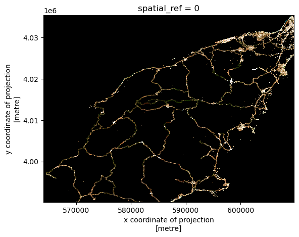
Figure 4
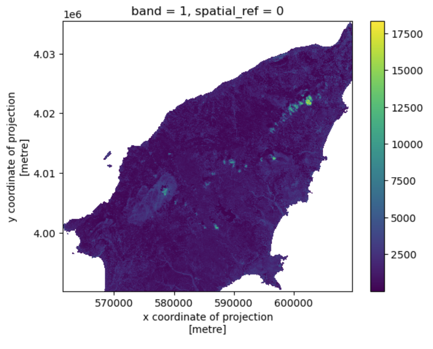
Figure 5
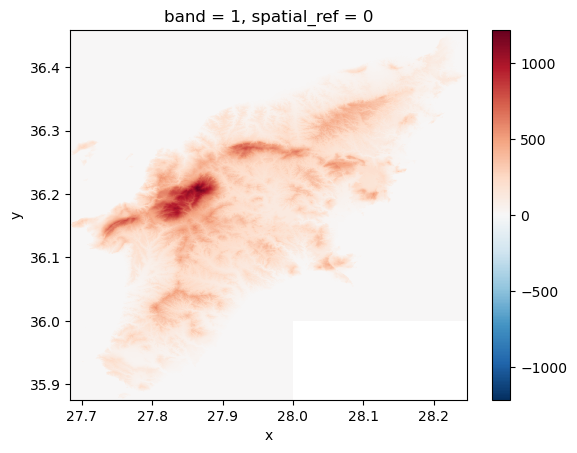
Figure 6
Raster Calculations in Python
Figure 1
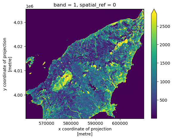
Figure 2
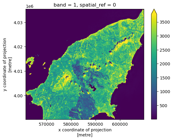
Figure 3
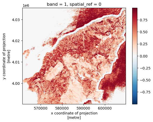
Figure 4
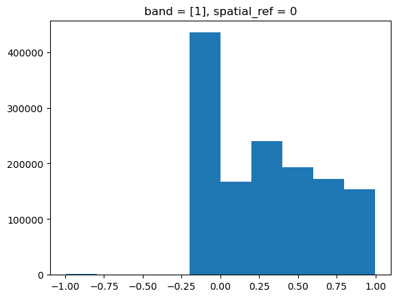
Figure 5
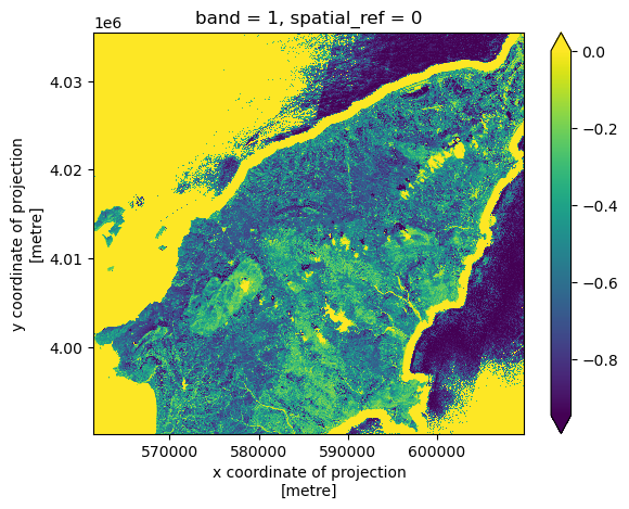
Figure 6
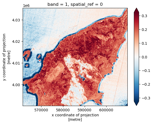
Figure 7
Calculating Zonal Statistics on Rasters
Figure 1
Parallel raster computations using Dask
Figure 1
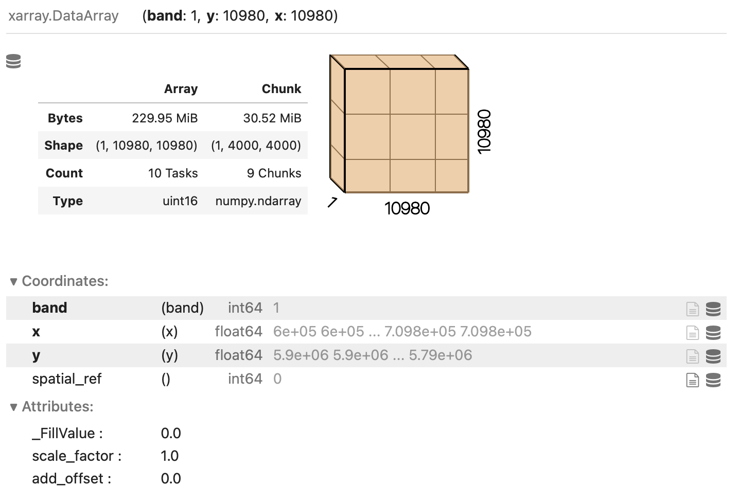
Xarray Dask-backed DataArray
Figure 2
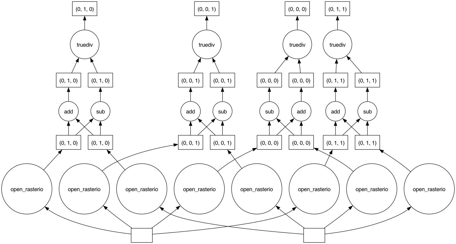
Dask graph
Data cubes with ODC-STAC
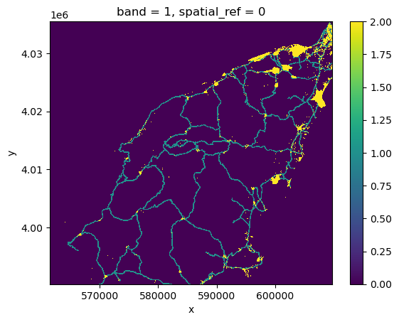
Figure 1
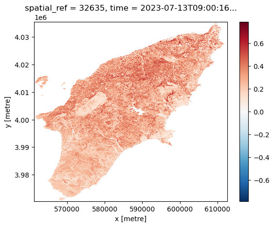
NDVI before the wildfire
Figure 2
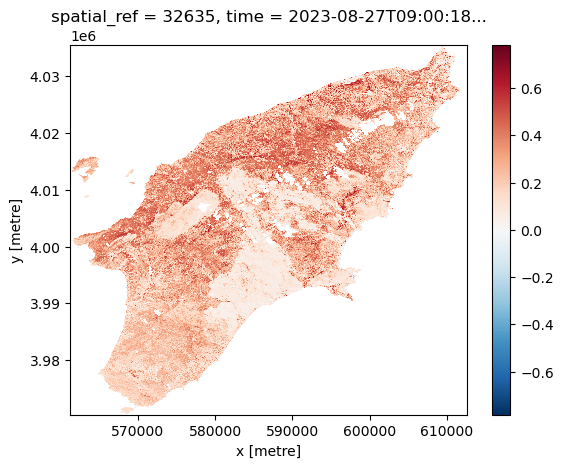
NDVI after the wildfire
Figure 3

NDVI plot with selected point
Figure 4
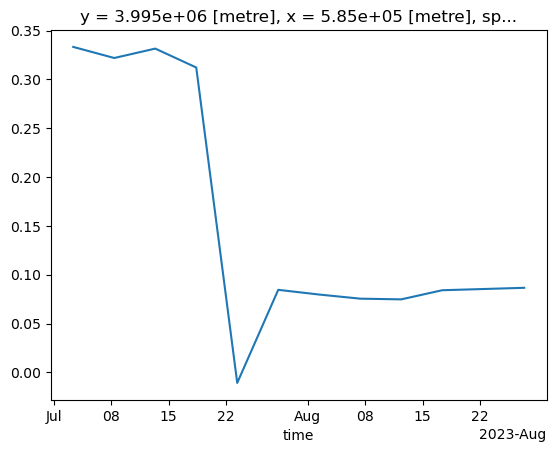
NDVI time series