Model coupling theory: the Multiscale Modelling and Simulation Framework
Last updated on 2022-10-31 | Edit this page
Overview
Questions
- When coupling models together, how do you figure out which information needs to be exchanged when?
- How does that depend on the spatial and temporal scales of the simulated processes?
- What does that mean for how submodels should be implemented?
Objectives
- Explain how to couple models using the concepts of the Multiscale Modelling and Simulation Framework
Introduction
Coupling models can be a difficult task, especially when there are many models involved that model processes in different ways and at different scales in time and space. To make a coupled simulation, you need to figure out which information needs to be passed between which submodels, when it needs to be sent and received, and how it can be represented, and that can be quite a puzzle. Fortunately, there is a theory of model coupling that can help you with this. It is called the Multiscale Modelling and Simulation Framework (MMSF), and despite its name, it also includes same-scale couplings.
In this episode, we’ll work through a slightly extended version of the MMSF’s process for coupling two models representing two processes.
Domains
Mathematical and simulation models represent some kind of process, which takes place in a certain location in time and in space: its domain. The weather takes place in the atmosphere, earthquakes in the Earth’s crust, a forest fire in a forest. In time, that forest fire begins with a lightning strike and ends when the flames are extinguished, and even continuous processes like the airflow around an aeroplane wing can be considered to start when circumstances change and end when a steady state is reached again.
The domains of two models can be the same, overlapping, adjacent, or separated, in both space and time. This is important for the coupling between them, because it decides what is sent (state or boundary conditions) and when it is sent.
Challenge 1: Models and domains
Think of two models that could potentially be coupled, and describe each model’s domain in time and space and the relation between them.
Some things to ponder:
- What does it mean for two models to have adjacent time domains?
- What if their spatial domains are separated?
Example coupled model
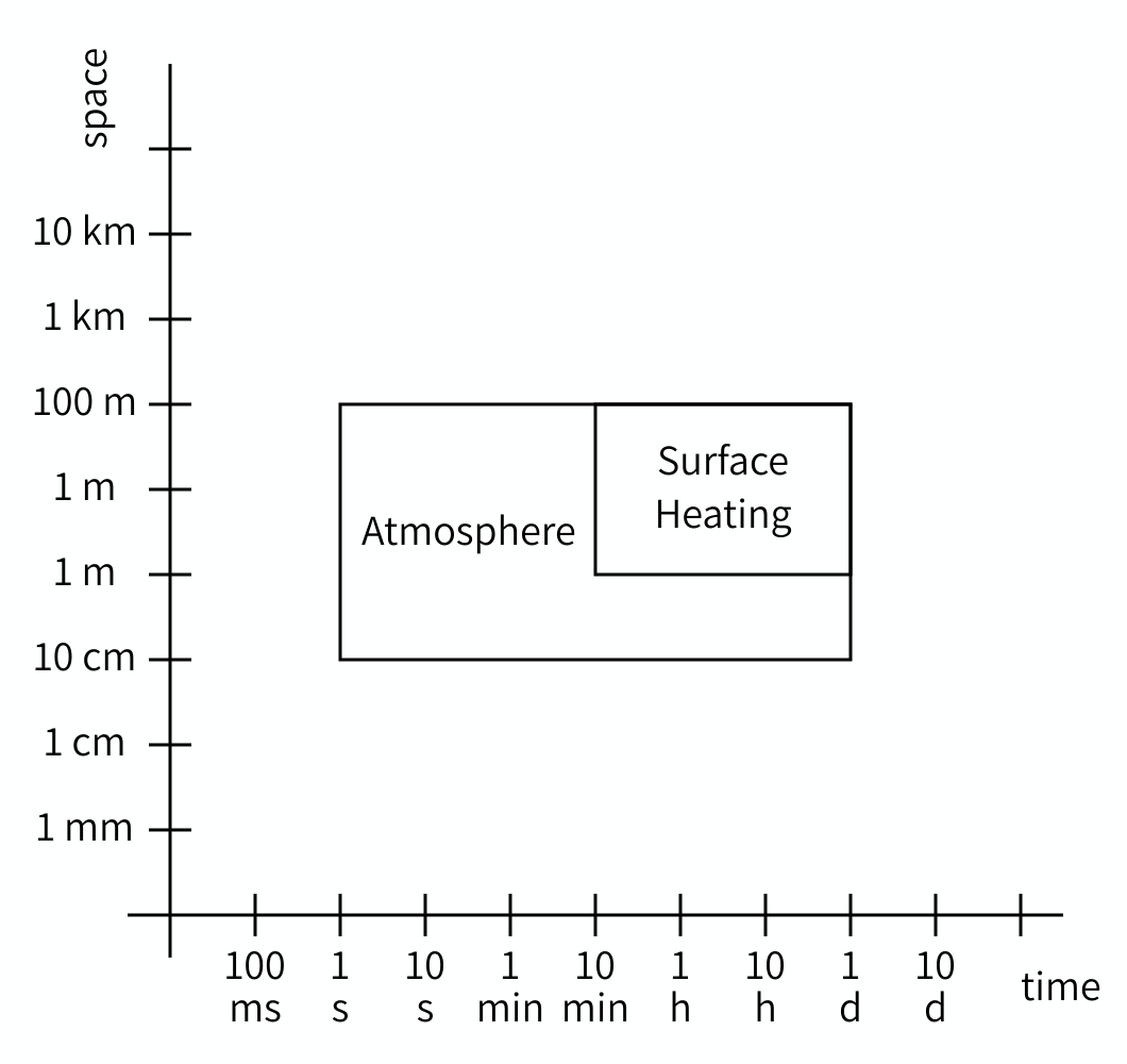
The sun drives local convection in the atmosphere by heating up the Earth’s surface, which then heats up the air above it. We can model how this plays out over the course of a day by coupling two models:
Model 1 simulates the heating of the Earth’s surface as the sun shines on it. Model 2 simulates the flow of the air above as it warms up and starts rising. In time, both domains extend from sunrise to sunset. In space, the heating process takes place on the Earth’s surface, while the airflow process operates on the atmosphere. In time, the domains overlap, while in space they are adjacent.
Questions
- If two models have adjacent time domains, then one model starts at the same moment that the other ends. Typically, this occurs when one process triggers another.
- If the spatial domains of two models are separated, then there is no direct exchange of information between the models, unless some kind of remote communication is possible. As a result, the models can be run separately and don’t need to be coupled, unless some other model has a domain adjacent to both.
Scales
A second important property of a physical process is the scales, again in time and in space, on which it takes place. A scale can be defined by its grain and extent. There are many other terms in use for these, but we’ll use these here because they’re less ambiguous than most. The grain refers to the smallest detail that the model can represent. In practice, that is usually set by the timestep (in time), grid spacing, or size of an agent (in space). If these can vary throughout the domain, pick the smallest. The extent refers to the size of the process in space and time, so the size of its domain. How long does it take to complete (or to reach a steady state), and how large an area is modelled?
Challenge 2: Models and scales
What are the scales of the models you previously considered the domains of? What are their grain and extent in space and in time?
Surface
Model 1 simulates the heating of the Earth’s surface as the sun shines on it.
The temperature of the Earth’s surface only changes slowly during the day, and we can probably say there are no significant changes from one minute to the next, or even for a somewhat larger interval. So the time grain of model 1 is on the order of a few minutes, perhaps up to an hour. The time extent of the model is one day, as it will repeat itself after that.
In space, the grain depends on the research question, and could be as small as 10 cm if we are looking at the detailed thermal environment around a building, or as large as a few kilometers if we want to make a national weather forecast. The extent is the size of the area of study.
Atmosphere
Model 2 simulates the flow of the air above as it warms up and starts rising. This is probably done using a computational fluid dynamics model. Both the temporal and spatial scales will depend on the research question here, and grains (time steps and grid spacing) may range from milliseconds and centimeters to minutes and kilometers. The spatial extent may be the same as that of Model 1, but it could be larger if a very tall column of air is modeled. In time, the atmosphere won’t reach a static equilibrium, but we could choose to run the simulation for the course of a day and use that as the temporal extent.
Note that you often cannot give an exact number, and that the scales are often something of a modeling decision. That’s usually alright, as we will see below.
Just like with domains, the scales of two models can be compared and their relation determined. The Scale Separation Map (SSM) is a nice tool for this. The SSM is a graph with on its horizontal axis a range of durations, and on its vertical axis a range of sizes. Each model can then be plotted as a box, with the left edge at the temporal grain, the right edge at the temporal extent, the lower edge at the spatial grain, and the upper edge at the spatial extent. Here is an example:
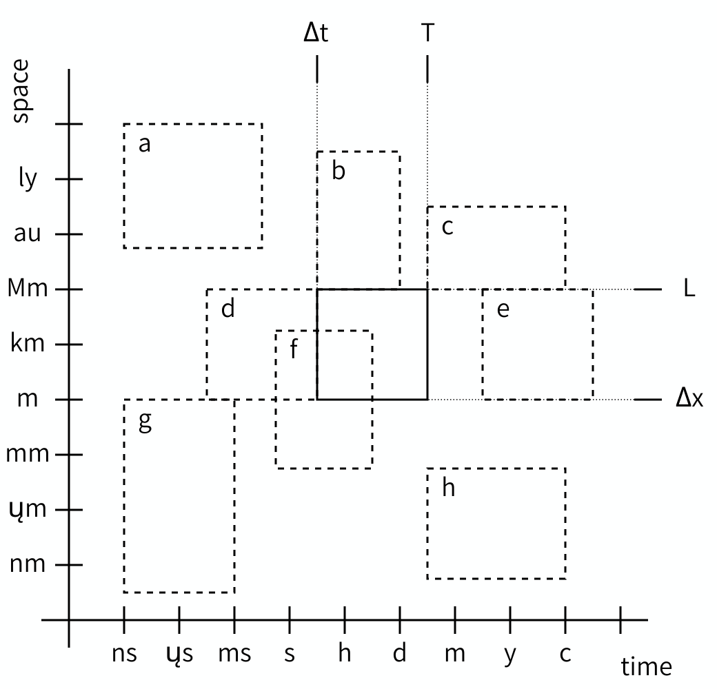
The SSM may look very counterintuitive at first, because we are used to plotting locations, not sizes. So look at the graph carefully and think about what you see and what it means. It does get easier to understand once you get the hang of it.
As you can see, we can plot multiple models on a Scale Separation Map and when we do, the map shows the relationship between the scales of two models. Both horizontally and vertically, model rectangles can have a gap between them (i.e. be separated), or be adjacent, or overlap, and the corresponding models are said to be scale separated, scale adjacent or scale overlapping in space and/or in time.
For coupling, it is actually only these relationships that matter. Even if you don’t know the exact grain or extent of a particular model, you can often decide whether it’s smaller, larger or the same as the grain or extent of another model and draw them correspondingly.
Challenge 3: Scale Separation Map
- What are the relations of scales a through h in the figure relative to the reference scale?
- Draw a scale separation map for the models you would like to couple.
Scale relations
- Spatially (larger) and temporally (faster) scale separated.
- Spatially scale adjacent (larger), temporally scale overlapping.
- Spatially scale adjacent (larger), temporally scale adjacent (larger).
- Spatially scale overlapping, temporally scale adjacent (smaller).
- Spatially scale overlapping, temporally scale separated (slower).
- Spatially and temporally scale overlapping.
- Spatially scale adjacent (smaller) and temporally scale separated (faster).
- Spatially scale separated (smaller) and temporally scale adjacent (slower).
Models and the Submodel Execution Loop
So far, we have talked about domains and scales of models, which we can do based on the physical properties of the modelled system, and the research questions we ask about that system. In order to be able to technically couple models however, we need to know what a model is. In the MMSF, this is done using a universal model-of-a-model called the Submodel Execution Loop (SEL):
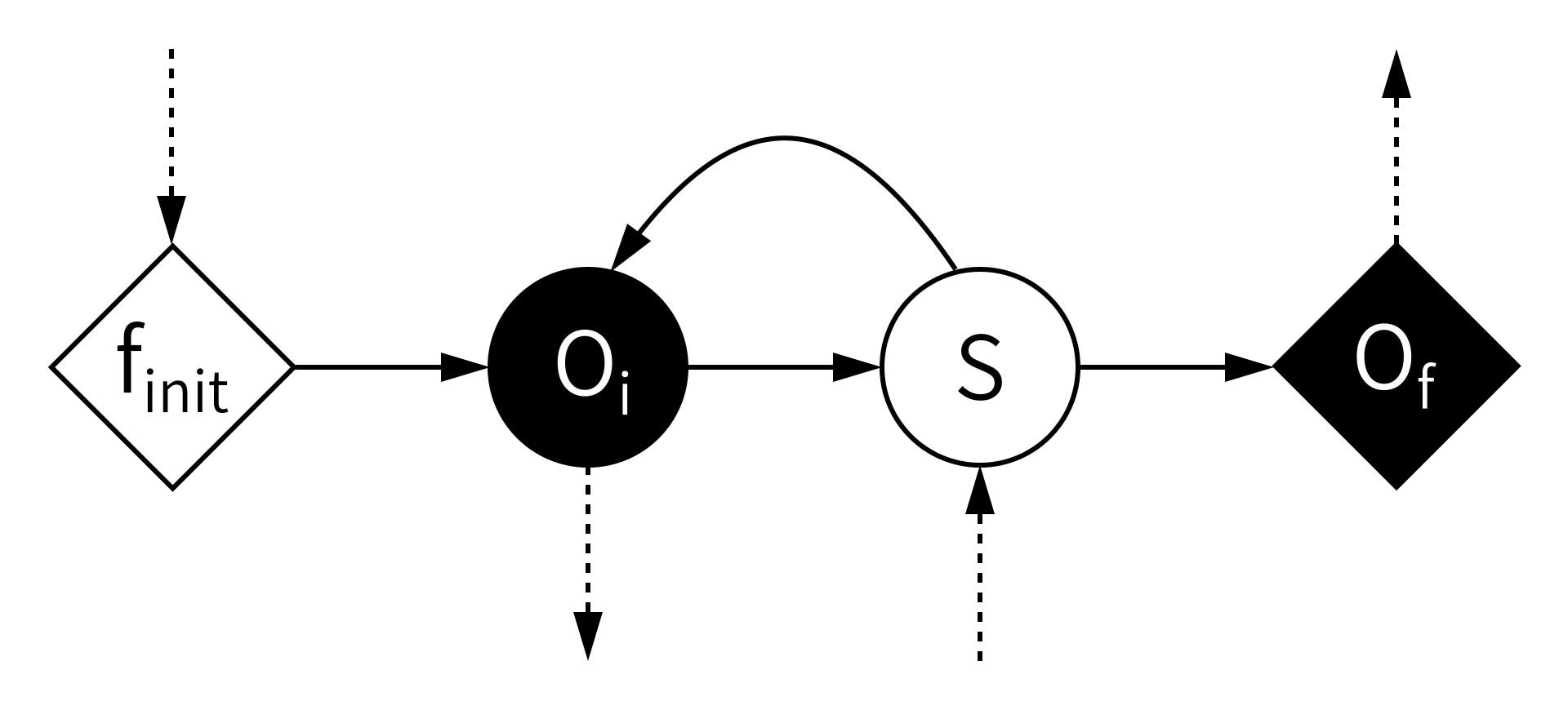
According to the MMSF, each model starts by initialising itself, a stage (or operator) known as \(f_{init}\). This puts the model into its initial state. During \(f_{init}\), information may be received from other models in a coupled simulation, which the model can use to initialise itself.
Second, some output based on that state is produced in the \(O_i\) operator. This is intermediate Output, or, looking from the outside in, we Observe an intermediate state, hence \(O_i\). This output may be sent to other models, where it can for example be used as boundary conditions.
Third, a state update may be performed using the \(S\) operator, which moves the model to its next state (timestep). During \(S\), information may be received from other models to help perform the state update.
After \(S\), the model may loop back to before \(O_i\), and repeat those two operators for a while, until the end of the time scale is reached. This leaves the model with a final state, which may be output in the \(O_f\) operator (for final output or observation).
Callout
Note that there’s a mnemonic here for the symbols: Operators \(O_i\) and \(S\), which are within the state update loop, have a circular symbol, while \(f_{init}\) and \(O_f\) use a diamond shape. Also, filled symbols designate ports on which messages are sent, while open symbols designate receiving ports. Information must always be sent from an operator with a filled symbol to one with an open symbol.
This basic model is quite flexible. If the loop is run zero times, then the model is a simple function. Timesteps may be of any length, and vary during the run, and the model may decide to stop and exit the state update loop at any time. The state may represent anything at all in any way, and it may be updated in whichever way is suitable for the model. Any simulation code you may want to use is very likely to fit these minimal constraints.
Temporal domain and scale relations
Now that we know what a model is and how models may be related in terms of their domains and scales, we can decide how to set up the coupled simulation. We do this by looking at all pairs of two models under consideration, one pair at a time, and consider the relationships between their temporal and spatial scales as well as their domains.
For reference, here are the possible relations between two time domains or two time scales:
| Property | Relation | Description |
|---|---|---|
| Domain | Same | At the same time, acting on the exact same bit of reality |
| Domain | Overlap | Some parts at the same time, acting on the same bit of reality |
| Domain | Adjacent | One starting precisely when the other ends |
| Domain | Separated | One starting some time after the other ends |
| Scale | Same | Same grain (dt) and extent (duration) |
| Scale | Overlap | Grain or extent differs, but neither model has a grain larger than the extent of the other or an extent smaller than the grain of the other |
| Scale | Adjacent | One model’s extent equals the other’s grain |
| Scale | Separated | One model’s extent is smaller than the other model’s grain |
Of the different properties, those governing time are the most interesting, and also potentially the most confusing. Let’s look at the possible scenarios one by one.
Adjacent or separated time domains
A simple case is when the time domains are adjacent, meaning one process starts right when the other process finishes, or separated, meaning one process starts some time after the other process finishes. In this case, the final output of the first model is used to initialise the subsequent model.
Same time domains and the same temporal scale
If two processes do not happen one after the other, then they occur at least partially simultaneously, and their models have overlapping time domains. The simplest among these cases is when the two processes start and end at the same time, and have the same timestep. In that case, each model updates its state to the next timestep, then sends some information based on the new state (e.g. boundary conditions) to the other model, receives information from the other model in return, and goes to do the next state update.
Same time domains and temporal scale separation
A third interesting case is when two processes happen at the same time, but one process is much faster than the other, so that it runs to completion in (much) less time than it takes the other to do a timestep. In that case, the fast model needs to do an entire run for every timestep of the slow model.
Challenge 4: Coupling Submodel Execution Loops
We can represent each of the two models in the scenarios above as a Submodel Execution Loop. To connect the models, we then have to send information between the operators of the models. For each of the three cases, figure out how to connect the Submodel Execution Loops of the two models so that the correct communication pattern is implemented.
If the time domains are adjacent or separated, then the final output of the first model is used to initialise the subsequent model. We can implement this by sending information from the first model’s \(O_f\) to the second model’s \(f_{init}\).
If the temporal scales are the same, then the models exchange information every time they have a new state. This can be done by connecting each model’s \(O_i\) to the other model’s \(S\), thus sending information at each step.
In case of temporal scale separation, the fast model needs to be reinitialised at every timestep of the slow model, do an entire run, and return some information based on its final state to the slow model. This can be accomplished by sending from the slow model’s \(O_i\) to the fast model’s \(f_{init}\) and from the fast model’s \(O_f\) back to the slow model’s \(S\).
Coupling Templates
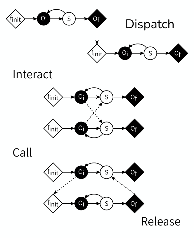
The three cases above demonstrate the four Coupling Templates defined by the MMSF. The first one, \(O_f\) to \(f_{init}\), is called dispatch. The second one, \(O_i\) to \(S\) is called interact, and usually comes in pairs. The third one and the fourth one usually go together, as the combination call (\(O_i\) to \(f_{init}\)) and release (\(O_f\) to \(S\)).
Given the constraints of which operators can send and which can receive, these are in fact all four possible types of connections, and between them they cover all kinds of temporal scale relations.
If the time domains or time scales overlap, but are not equivalent, then an additional component is needed that sits between the models; we will not go into that advanced use case here.
Spatial domains, scales and multiplicity
Having discussed temporal scales, let’s move on to the spatial scales. Like with scales in time, scales in space can be the same, overlap, be adjacent or be separated, and you can see which one you have by looking at your Scale Separation Map. Here’s another table with the interpretation of those relations in space:
| Property | Relation | Description |
|---|---|---|
| Domain | Same | In the same place, acting on the exact same bit of reality |
| Domain | Overlap | Some parts in the same place, acting on the same bit of reality |
| Domain | Adjacent | Acting on two different bits of reality which touch each other (space) |
| Domain | Separated | Acting on two different bits of reality which do not touch (space) |
| Scale | Same | Same grain (dx) and extent (size) |
| Scale | Overlap | Grain or extent differs, but neither model has a grain larger than the extent of the other or an extent smaller than the grain of the other |
| Scale | Adjacent | One model’s extent equals the other’s grain |
| Scale | Separated | One model’s extent is smaller than the other model’s grain |
Same spatial domain and scale
This is a very tight coupling, where usually the two processes end up in a single equation on the theory side, and in a single code in the implementation. Unless there is temporal scale separation, it’s probably better to combine the models into a single implementation. In case of temporal scale separation, a call-and-release template may be used and the state is passed back and forth between the models.
Same spatial domain, adjacent or separated scales
If one process is much smaller than the other, then the entire small process takes place within one grid cell or agent of the larger process. Frequently, this means that there are multiple instances of the smaller model, maybe even one for each grid cell or agent, with communication between the large-scale model and each small-scale model instance. Some kind of iterative equilibration between the models may be needed to reconcile the two representations of the state.
Adjacent spatial domains, same or overlapping spatial scales
If two processes are of similar size and resolution, but occur on adjacent domains, then they will each have their own state, and exchange boundary conditions. If there’s a temporal scale separation between them, then the call-and-release coupling template is used and the called (fast) model keeps its state in between calls.
Challenge 5: Spatial relations
Think of an example for each of the above spatial domain and scale relations. Can you think of examples that don’t fit any of them?
- Reaction-diffusion models have the two processes acting on the same domain and spatial scale, but may be temporally scale-separated depending on parameter values.
- A crack propagation model coupling a continuum representation of a material sample to molecular mechanics models at specific points. Stresses and strains are exchanged in this case.
- In a simulation of In-Stent Restenosis, a complication of vascular surgery, a cell growth process in the wall of an artery is coupled with a fluid dynamics simulation of the blood flow through the artery. The domains are adjacent and boundary conditions are exchanged.
MMSL Diagrams
For larger coupled simulations consisting of several submodels and other components, drawing the complete submodel execution loop as we did above gets too complicated. Fortunately, a simplified notation is available in the form of the Multiscale Modelling and Simulation Language (MMSL). This language describes a coupled simulation as a set of components and the connections between them. Its YAML-based form, yMMSL, is used as the configuration language for MUSCLE3 (more on which in the next episodes). Its graphical form, gMMSL, provides a compact visual representation of a coupled model:
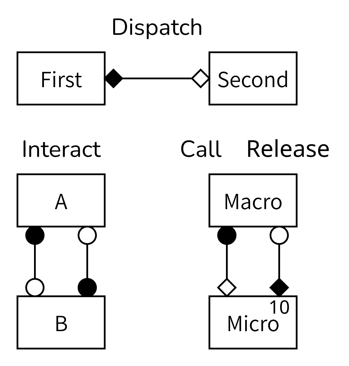
Challenge 6: Deciphering gMMSL
Explain the above figure.
Each box represents a submodel. The lines show where information is sent from one model to another. The diamonds and circles designate the SEL operators that information is sent from and to. A number in the top right corner of a box is optional, but when it’s there it shows how many instances of that submodel exist. In this case, the model at the bottom right has temporal and spatial scale separation, so it uses the call-and-release coupling template and has multiple instances of the micromodel.
Note that there can be multiple lines or conduits between the same operators and models if multiple bits of information need to be transferred, but then these could also be glued together into a single message. This is a modelling decision, so do what works best for your model.
Not shown in the diagram is that the lines can be labeled with a label at each end showing the name of the port on the model that is being connected. Especially if there are multiple lines then it is necessary to do that to avoid confusion. More about this in the following episodes, when we connect two models using MUSCLE3.
Callout
Real simulations often need more than just the submodels, especially if you want to keep everything nice and modular. Different models often send and receive data in different formats for example, so that you need converters, and sometimes splitters and joiners that can split messages or join them together. If there is a scale difference, then some kind of scale bridge usually needs to be implemented, and for uncertainty quantification components may be needed that sample parameters and combine results into distributions.
These components are often simple functions, and can then be implemented just like a submodel with only an \(f_{init}\) and \(O_f\). Such a component can then be inserted in between a connection between two submodels by interrupting a conduit and putting it in between.
Key Points
- Physical processes take place on a domain and at certain scales in time and space
- Simulation models are described by the Submodel Execution Loop
- Given two models and their domains and scales, we can decide which coupling template to use to connect them
- An MMSL diagram can be used to visualise a complete coupled simulation