MUSCLE3 - coupling and running

Overview

Questions

• How do you couple multiple sub-models using MUSCLE3?
• How do you run a coupled simulation with MUSCLE3?

Objectives

• Demonstrate how MUSCLE3 implements the Multiscale Modelling and Simulation Language (MMSL)
• Configure a coupled simulation with MUSCLE3
• Run a coupled simulation using MUSCLE3

Introduction

---

We managed to connect one of our sub-models, the reaction model, to MUSCLE. In order to make a coupled simulation, we need at least two models. The second model here is the diffusion model. We prepared it for you, adding the necessary MUSCLE bindings and comments similar to what we did for the reaction model. You can open it from diffusion.py.

Investigating the macro model

---

Challenge 1: Investigating the diffusion model

The diffusion.py file contains a couple of functions, as well as a few lines of code that may come in useful later. For now, let’s focus on the diffusion function.

• Compared to the reaction function you made previously, what is different, other than the mathematics of the model itself?

Show me the solution

• The ports are named differently, and are attached to different operators
• The send and receive statements are now within the state update loop

Connecting the models together

---

With both models defined, we now need to instruct MUSCLE3 on how to connect them together. Recall the gMMSL diagram from the previous episode (with port names, this time):

gMMSL diagram for the reaction-diffusion model

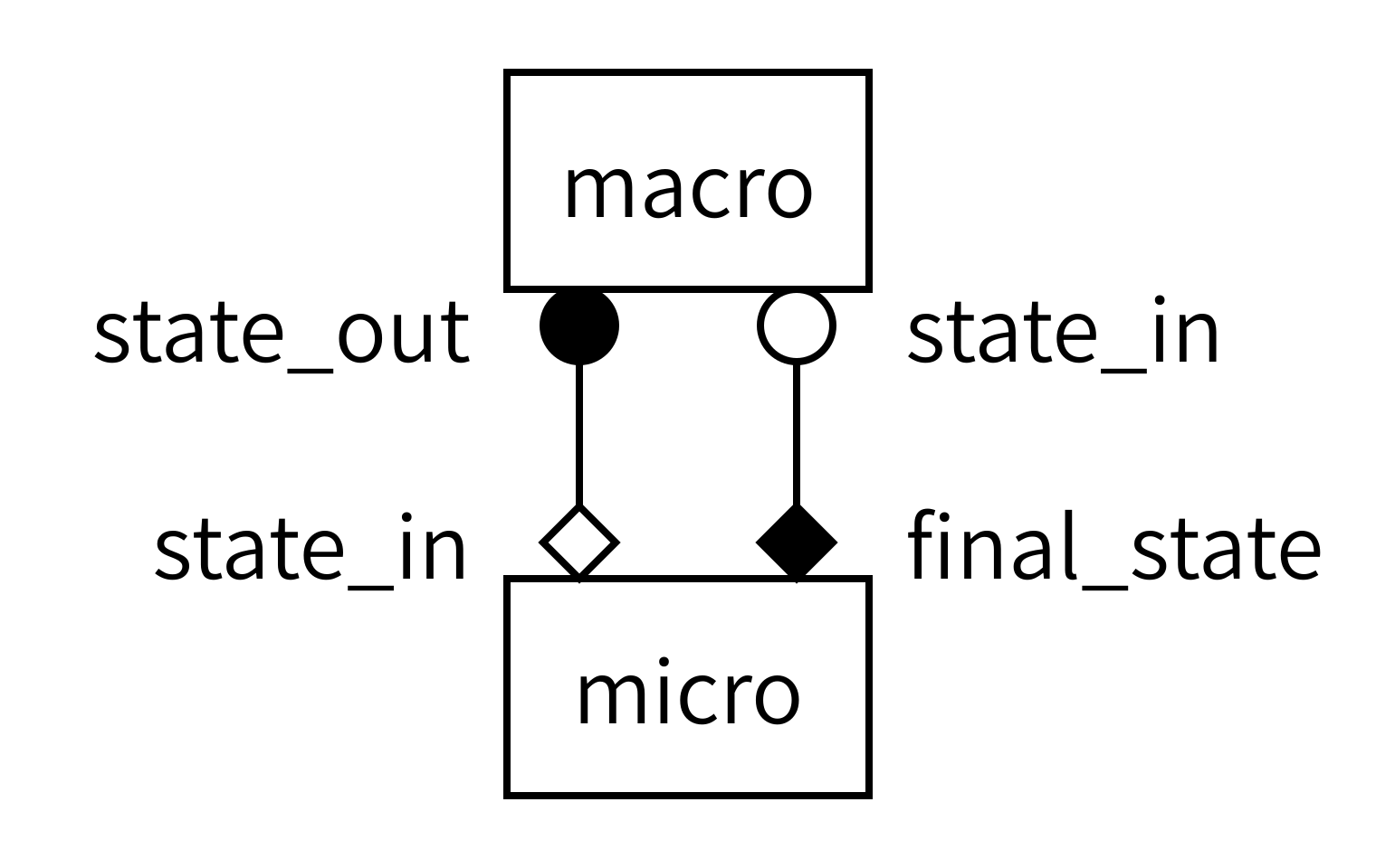
Since diagrams aren’t valid Python, we need an alternative way of describing this model in our code. For this, we will create a MUSCLE configuration file written in the yMMSL language. This file tells the MUSCLE manager about the existence of each submodel and how it should be connected to the other components.

Challenge 2: Creating the yMMSL file

Open the file reaction_diffusion.ymmsl. In it, you’ll find an incomplete yMMSL description of the coupled simulation, as shown below. Your challenge? Complete it!

Tip: remember that this is a textual description of the diagram above. All the information you need is in there.

YAML

ymmsl_version: v0.1

model:
  name: reaction_diffusion

  components:
    macro:
      implementation: diffusion
      ports:
        o_i: state_out
        ...

    ...
      implementation: reaction
      ...

  conduits:
    macro.state_out: micro.initial_state
    ...

Show me the solution

YAML

ymmsl_version: v0.1

model:
  name: reaction_diffusion_python

  components:
    macro:
      implementation: diffusion
      ports:
        o_i: state_out
        s: state_in

    micro:
      implementation: reaction
      ports:
        f_init: initial_state
        o_f: final_state

  conduits:
    macro.state_out: micro.initial_state
    micro.final_state: macro.state_in

First, we describe the two components in this model. Components can be submodels, or helper components that convert data, control the simulation, or otherwise implement required non-model functionality. The name of a component is used by MUSCLE as an address for communication between the models. The implementation name is intended for use by a launcher, which would start the corresponding program to create an instance of a component. It is these instances that form the actual running simulation. In this example, we have two submodels: one named macro and one named micro. Macro is implemented by an implementation named diffusion, while micro is implemented by an implementation named reaction.

Second, we need to connect the components together. This is done by conduits, which have a sender and a receiver. Here, we connect sending port state_out on component macro to receiving port initial_state on component micro.

Adding settings

---

The above specifies which submodels we have and how they are connected together. Next, we need to configure them by adding the settings to the yMMSL file. These will be passed to the models, who get them using the Instance.get_settings() function. Go ahead and add them to your reaction_diffusion.ymmsl:

YAML

settings:
  micro.t_max: 2.469136e-6
  micro.dt: 2.469136e-8
  macro.t_max: 1.234568e-4
  macro.dt: 2.469136e-6
  x_max: 1.01
  dx: 0.01
  k: -4.05e4    # reaction parameter
  d: 4.05e-2    # diffusion parameter

Look at the names of the settings. Does anything stand out to you?

Specifying resources

---

Finally, we need to tell MUSCLE3 whether and if so how each model is parallelised, so that it can reserve adequate resources for each component. In this case, the models are single-threaded so that is what we specify. Again, add this to your file.

YAML

resources:
  macro:
    threads: 1
  micro:
    threads: 1

Note that we specify resources for each component, not for each implementation.

Launching the simulation

---

This gives us all the pieces needed to construct a coupled simulation. All we need is the two model functions and the configuration, then we can connect them together and run the whole thing. The model functions we can import from the files we saw before:

PYTHON

from diffusion import diffusion
from reaction import reaction

To load the configuration, we use the load() function from the ymmsl module that comes with MUSCLE3:

PYTHON

from pathlib import Path
import ymmsl

configuration = ymmsl.load(Path('reaction_diffusion.ymmsl'))

Finally, we need to create a connection from the names of the implementations listed in the yMMSL file to the Python functions that are those implementations:

PYTHON

implementations = {'reaction': reaction, 'diffusion': diffusion}

And then we can ask MUSCLE3 to start the coupled simulation:

PYTHON

from libmuscle.runner import run_simulation.

run_simulation(configuration, implementations)

You will find a coupled_model.py file with the others, which implements the above. It also configures Python’s logging subsystem to give us a bit more log output.

Challenge 3: Running the coupled simulation

If you haven’t already done so, add the settings and resources to your reaction_diffusion.ymmsl. Then, have a look at the coupled_model.py script and see if you can run it. It should show a plot on the screen showing the concentration over time. If not, try to find the problem! You should have a muscle_manager.log file, and maybe a muscle3.micro.log and muscle3.macro.log to help you figure out what went wrong.

Show me the solution

$ python3 coupled_model.py

Running separate programs using the MUSCLE3 manager

---

The above coupled_model.py script imports the models as Python functions, and then starts them using MUSCLE3’s runner.run_simulation() function. This works great for models consisting entirely of Python components, and which are small enough to run on the local machine. However, models written in other languages like C++ or Fortran cannot be imported as Python functions, and larger simulations may need to run on many nodes on an HPC cluster. For such simulations, we cannot use run_simulation(), and we need to use the MUSCLE3 manager instead.

The MUSCLE3 manager, like the runner, gets a model description and a list of implementations to use, and then starts each required instance by starting its implementation. That’s a fair bit of new terminology, so here is what those words mean:

Component

Represents a simulated process with a domain and a scale, or is a helper component. One box in the gMMSL diagram. May have a single instance, or multiple instances e.g. in case of spatial scale separation or if it’s part of a UQ ensemble.

Instance

A running program simulating a particular component. This may be a parallel program running on many cores or across many machines, or in could be a simple Python script.

Implementation

A computer program (e.g. a Python script) that can be started to create an instance.

Challenge 4: Running using the manager

In this final challenge, we’ll run the reaction-diffusion model using the MUSCLE3 manager. This takes three steps: turning the reaction model into a stand-alone program, telling the manager how to start the programs, and finally running it all.

Create a stand-alone Python program

First, you need to turn reaction.py into a stand-alone Python program.

Hint: Look at diffusion.py, which is already set up to do this. You can copy-paste and adapt from there.

Add an implementations section

Next, you need to add an implementations: section to your yMMSL file. The implementations section describes which implementations are available to run. Here’s a template for a Python program:

implementations:
  <implementation_name>:
    virtual_env: <absolute path to virtual env to load>
    executable: python
    args: <absolute path to Python script>

Add this section to your reaction_diffusion.ymmsl, and replace all the items in angle brackets with the correct values.

Run the simulation

To run the simulation using the manager, open a terminal and activate the virtual environment in which you’ve installed MUSCLE3. You can then start the simulation using muscle_manager --start-all reaction_diffusion.ymmsl. Do that, and inspect the output!

Show me the solution

To turn reaction.py into a stand-alone program, you need to add the final section of diffusion.py to the end, slightly modified:

if __name__ == '__main__':
    logging.basicConfig()
    logging.getLogger().setLevel(logging.INFO)
    reaction()

The yMMSL file then gets an implementations section like this:

implementations:
  reaction:
    virtual_env: /path/to/workdir/env
    executable: python
    args: /path/to/workdir/reaction.py

  diffusion:
    virtual_env: /path/to/workdir/env
    executable: python
    args: /path/to/workdir/diffusion.py

Then, you can run using

(env) $ muscle_manager --start-all reaction_diffusion.ymmsl

And that will create a directory named run_reaction_diffusion_<date>_<time> with all the log files and model output neatly organised.

Key Points

• Models may differ in which ports they have and when they send and receive
• The yMMSL file discribes components, conduits, settings and resources
• Running the coupled simulation can be done from a Python script
• For larger simulations and C++ and Fortran, submodels run as separate programs via the MUSCLE3 manager