Content from Introduction to model coupling

---

Last updated on 2022-10-31 | Edit this page

Overview

Questions

• What is meant by a “model”?
• What is the difference between a mathematical model and a computational model?
• What is model coupling?
• Why would we want to couple simulation models?

Objectives

• Explain the benefits of coupling simulation models

Introduction

---

Computer simulations are widely used in modern science to understand and predict the behaviour of natural systems. The computer program that simulates a given physical system is referred to as a model of that system. For example, a climate simulation code is a model of the Earth’s climate. Some models may be very simple e.g. describing the evolution of a 1 dimensional system. Others may be highly complex, involving many different physical processes. A well known use of computer simulation is in the field of weather forecasting, in which a very complex model composed of a multitude of different physical processes must be simulated by a computer program, generally requiring powerful supercomputers.

Mathematical model vs computational model

---

For this course, it is important to distinguish between a mathematical model, and a computational model. A mathematical model refers to the set of mathematical equations that describe the evolution of a given physical system. The computational model refers to the actual computer program that describes the evolution of a physical system. These are closely connected concepts - after all, many computational models are just solving a given mathematical model numerically. However, the distinction is important. Some computational models can be simulating many different aspects of a physical system, which could involve solving many different mathematical models. The process of making sure that a computational model is solving the mathematical model you think it is, is called verification.

What is model coupling?

---

In short, “coupling” one computational model to another means that we pass information between the models in order to connect them into one big model. If the output of one model can be used as the input of another, for example, then it may be possible to couple them. The models must of course be compatible - at least one model must calculate something that can be used by the other model.

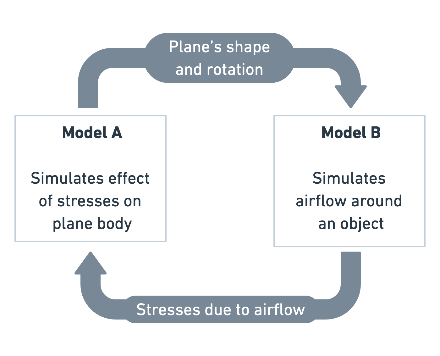
An example: Making a coupled model of a flying aeroplane

Imagine that we wish to simulate a flying aeroplane, but we only have two separate models: Model A and Model B.

Computational fluid dynamics solver applied to A380 aircraft. (Image: DLR, CC-BY 3.0)

Model A simulates how an aeroplane moves in response to forces on its body. Model B simulates airflow around objects and calculates the forces generated by that airflow. We could pass the shape, speed and rotation of the airplane as input to Model B, allowing it to calculate the forces on the plane. In turn, we could then pass the calculated forces back to Model A, allowing it to calculate the effect of the forces on the plane’s speed, position and rotation. In this way we have coupled the two models together, making a new, more complex computational model. The two original models are submodels of the coupled model.

Models A and B for the plane coupling example

Exercise: Breaking it down

Think of another system you might want to simulate. Can you think of how to break it down into two or more computational submodels? Most importantly, consider what information would be passed from one model to the other.

Example solution

• Local climate-ecology: One model simulates the expected climate of a region of the Earth under certain vegetation/land use conditions. A separate model simulates the proliferation and behaviour of animals and vegetation in a given region under influence of various climatic conditions.
• Stent in a blood vessel: There is a computational fluid dynamics model (simulating the blood flow) through a stent. A separate model is modelling the growth of scar tissue, that covers the stent as the artery wall heals. The stresses created by the blood on the stent and tissue affect how it grows. In turn, the new, narrowed arterial wall needs to be passed back to the blood flow model, since new tissue will affect the flow.

Why couple models together?

---

It is generally simpler and cheaper to simulate a small part of a system, or specific physical interaction. Processes at different length or time scales are often subject to different forces, while they can neglect others. For example, a mechanical model of a car frame will not consider behaviour at the atomic scale, whereas a molecular dynamics simulation naturally must. Computational modelling is therefore often highly specialised.

Furthermore, there can be an enormous number of different computational models even for the same problem, at the same length and time scales. Some models may be more accurate than others, or include newer theory etc. A scientist or engineer will combine different submodels together to run different computational experiments.

Why bother? Let’s just have one big model

Rather than couple existing models together, it is of course possible to simply create a single, monolithic model that handles all of the interactions within it. Can you think of reasons why we would not want to do that?

Show me the solution

• Code re-use: If a model already exists then ideally you should reuse it, rather than re-invent the wheel.
• Separation of concerns: The submodel does ‘one thing and does it well’ (hopefully). The modularity of keeping code separate in this way can really help with long term maintenance of a large comple simulation model. This is particularly obvious when models simulate processes that happen on totally different and non-overlapping length and time scales.
• Speed of building new models: If people can construct a complex model out of smaller, highly tested and optimised building blocks, then the task is a lot less laborious.
• Ease of swapping new, different models in and out. If a new, faster or more accurate implementation of a model is released, you want to be able to swap out an existing submodel for it. Having everything in a single monolithic code can lead to a tangled mess that is harder to refactor. In many cases it will just not be worth the time to refactor the existing simulation code, and people will write a new one, or not try the new model at all.
• Performance: A model coupling approach often makes it easier to exploit the massive parallelism of supercomputers.

Key Points

• Crossing the scales
• Modularity
• Flexibility
• Performance

Content from Model coupling theory: the Multiscale Modelling and Simulation Framework

---

Last updated on 2022-10-31 | Edit this page

Overview

Questions

• When coupling models together, how do you figure out which information needs to be exchanged when?
• How does that depend on the spatial and temporal scales of the simulated processes?
• What does that mean for how submodels should be implemented?

Objectives

• Explain how to couple models using the concepts of the Multiscale Modelling and Simulation Framework

Introduction

---

Coupling models can be a difficult task, especially when there are many models involved that model processes in different ways and at different scales in time and space. To make a coupled simulation, you need to figure out which information needs to be passed between which submodels, when it needs to be sent and received, and how it can be represented, and that can be quite a puzzle. Fortunately, there is a theory of model coupling that can help you with this. It is called the Multiscale Modelling and Simulation Framework (MMSF), and despite its name, it also includes same-scale couplings.

In this episode, we’ll work through a slightly extended version of the MMSF’s process for coupling two models representing two processes.

Domains

---

Mathematical and simulation models represent some kind of process, which takes place in a certain location in time and in space: its domain. The weather takes place in the atmosphere, earthquakes in the Earth’s crust, a forest fire in a forest. In time, that forest fire begins with a lightning strike and ends when the flames are extinguished, and even continuous processes like the airflow around an aeroplane wing can be considered to start when circumstances change and end when a steady state is reached again.

The domains of two models can be the same, overlapping, adjacent, or separated, in both space and time. This is important for the coupling between them, because it decides what is sent (state or boundary conditions) and when it is sent.

Challenge 1: Models and domains

Think of two models that could potentially be coupled, and describe each model’s domain in time and space and the relation between them.

Some things to ponder:

• What does it mean for two models to have adjacent time domains?
• What if their spatial domains are separated?

Example solution

Example coupled model

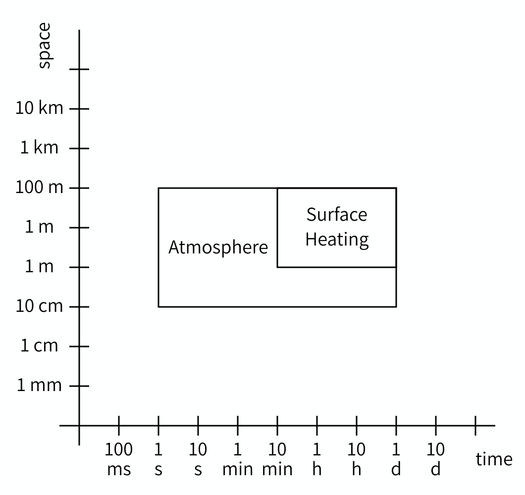
The sun drives local convection in the atmosphere by heating up the Earth’s surface, which then heats up the air above it. We can model how this plays out over the course of a day by coupling two models:

Model 1 simulates the heating of the Earth’s surface as the sun shines on it. Model 2 simulates the flow of the air above as it warms up and starts rising. In time, both domains extend from sunrise to sunset. In space, the heating process takes place on the Earth’s surface, while the airflow process operates on the atmosphere. In time, the domains overlap, while in space they are adjacent.

Questions

• If two models have adjacent time domains, then one model starts at the same moment that the other ends. Typically, this occurs when one process triggers another.
• If the spatial domains of two models are separated, then there is no direct exchange of information between the models, unless some kind of remote communication is possible. As a result, the models can be run separately and don’t need to be coupled, unless some other model has a domain adjacent to both.

Scales

---

A second important property of a physical process is the scales, again in time and in space, on which it takes place. A scale can be defined by its grain and extent. There are many other terms in use for these, but we’ll use these here because they’re less ambiguous than most. The grain refers to the smallest detail that the model can represent. In practice, that is usually set by the timestep (in time), grid spacing, or size of an agent (in space). If these can vary throughout the domain, pick the smallest. The extent refers to the size of the process in space and time, so the size of its domain. How long does it take to complete (or to reach a steady state), and how large an area is modelled?

Challenge 2: Models and scales

What are the scales of the models you previously considered the domains of? What are their grain and extent in space and in time?

Example solution

Surface

Model 1 simulates the heating of the Earth’s surface as the sun shines on it.

The temperature of the Earth’s surface only changes slowly during the day, and we can probably say there are no significant changes from one minute to the next, or even for a somewhat larger interval. So the time grain of model 1 is on the order of a few minutes, perhaps up to an hour. The time extent of the model is one day, as it will repeat itself after that.

In space, the grain depends on the research question, and could be as small as 10 cm if we are looking at the detailed thermal environment around a building, or as large as a few kilometers if we want to make a national weather forecast. The extent is the size of the area of study.

Atmosphere

Model 2 simulates the flow of the air above as it warms up and starts rising. This is probably done using a computational fluid dynamics model. Both the temporal and spatial scales will depend on the research question here, and grains (time steps and grid spacing) may range from milliseconds and centimeters to minutes and kilometers. The spatial extent may be the same as that of Model 1, but it could be larger if a very tall column of air is modeled. In time, the atmosphere won’t reach a static equilibrium, but we could choose to run the simulation for the course of a day and use that as the temporal extent.

Note that you often cannot give an exact number, and that the scales are often something of a modeling decision. That’s usually alright, as we will see below.

Just like with domains, the scales of two models can be compared and their relation determined. The Scale Separation Map (SSM) is a nice tool for this. The SSM is a graph with on its horizontal axis a range of durations, and on its vertical axis a range of sizes. Each model can then be plotted as a box, with the left edge at the temporal grain, the right edge at the temporal extent, the lower edge at the spatial grain, and the upper edge at the spatial extent. Here is an example:

The Scale Separation Map. The box in the center depicts the scale of a given process or model, the dashed boxes show possible other scales and the corresponding relationships.

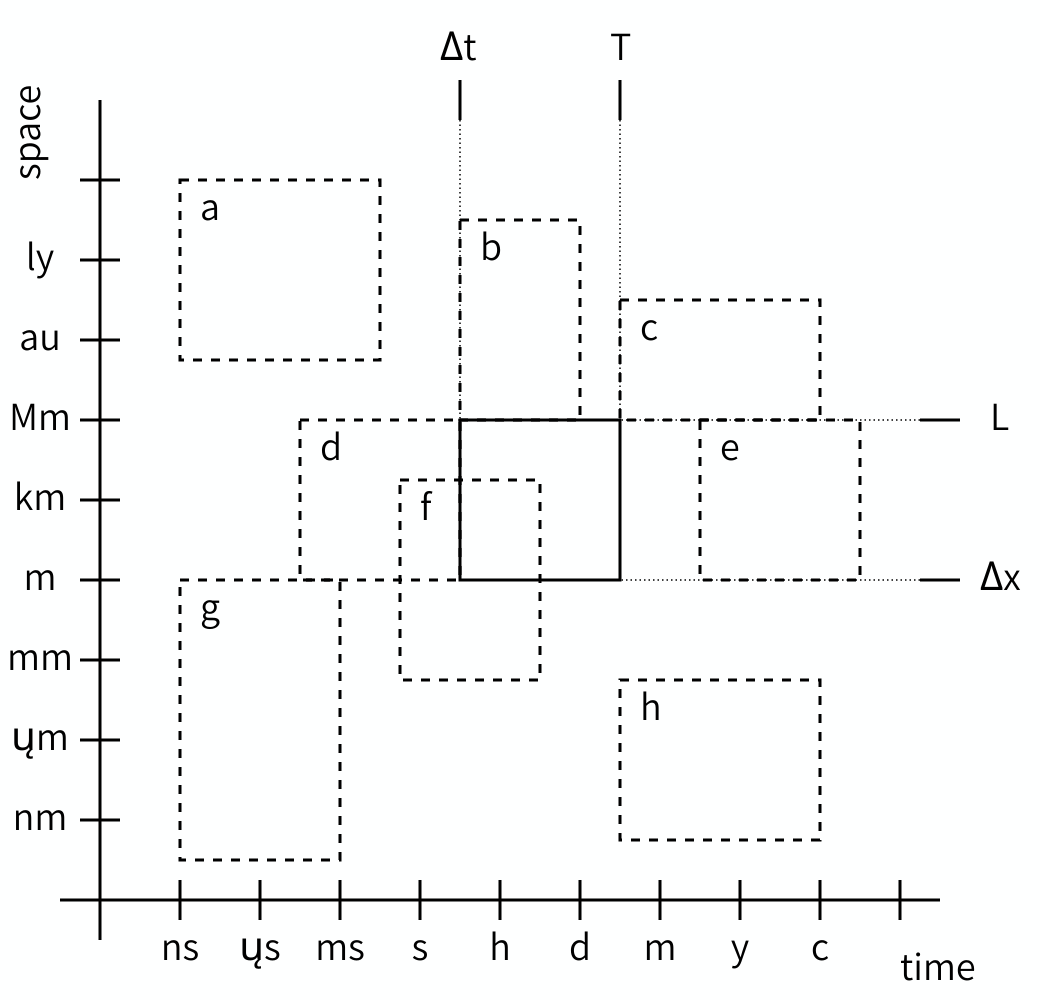
The SSM may look very counterintuitive at first, because we are used to plotting locations, not sizes. So look at the graph carefully and think about what you see and what it means. It does get easier to understand once you get the hang of it.

As you can see, we can plot multiple models on a Scale Separation Map and when we do, the map shows the relationship between the scales of two models. Both horizontally and vertically, model rectangles can have a gap between them (i.e. be separated), or be adjacent, or overlap, and the corresponding models are said to be scale separated, scale adjacent or scale overlapping in space and/or in time.

For coupling, it is actually only these relationships that matter. Even if you don’t know the exact grain or extent of a particular model, you can often decide whether it’s smaller, larger or the same as the grain or extent of another model and draw them correspondingly.

Challenge 3: Scale Separation Map

• What are the relations of scales a through h in the figure relative to the reference scale?
• Draw a scale separation map for the models you would like to couple.

Example solution

Scale relations

1. Spatially (larger) and temporally (faster) scale separated.
2. Spatially scale adjacent (larger), temporally scale overlapping.
3. Spatially scale adjacent (larger), temporally scale adjacent (larger).
4. Spatially scale overlapping, temporally scale adjacent (smaller).
5. Spatially scale overlapping, temporally scale separated (slower).
6. Spatially and temporally scale overlapping.
7. Spatially scale adjacent (smaller) and temporally scale separated (faster).
8. Spatially scale separated (smaller) and temporally scale adjacent (slower).

Scale Separation Map

Scale Separation Map for the atmosphere/surface model.

Models and the Submodel Execution Loop

---

So far, we have talked about domains and scales of models, which we can do based on the physical properties of the modelled system, and the research questions we ask about that system. In order to be able to technically couple models however, we need to know what a model is. In the MMSF, this is done using a universal model-of-a-model called the Submodel Execution Loop (SEL):

Submodel Execution Loop (SEL)

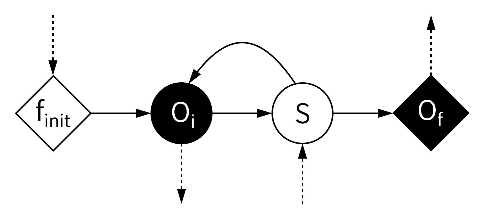
According to the MMSF, each model starts by initialising itself, a stage (or operator) known as \(f_{init}\). This puts the model into its initial state. During \(f_{init}\), information may be received from other models in a coupled simulation, which the model can use to initialise itself.

Second, some output based on that state is produced in the \(O_i\) operator. This is intermediate Output, or, looking from the outside in, we Observe an intermediate state, hence \(O_i\). This output may be sent to other models, where it can for example be used as boundary conditions.

Third, a state update may be performed using the \(S\) operator, which moves the model to its next state (timestep). During \(S\), information may be received from other models to help perform the state update.

After \(S\), the model may loop back to before \(O_i\), and repeat those two operators for a while, until the end of the time scale is reached. This leaves the model with a final state, which may be output in the \(O_f\) operator (for final output or observation).

Callout

Note that there’s a mnemonic here for the symbols: Operators \(O_i\) and \(S\), which are within the state update loop, have a circular symbol, while \(f_{init}\) and \(O_f\) use a diamond shape. Also, filled symbols designate ports on which messages are sent, while open symbols designate receiving ports. Information must always be sent from an operator with a filled symbol to one with an open symbol.

This basic model is quite flexible. If the loop is run zero times, then the model is a simple function. Timesteps may be of any length, and vary during the run, and the model may decide to stop and exit the state update loop at any time. The state may represent anything at all in any way, and it may be updated in whichever way is suitable for the model. Any simulation code you may want to use is very likely to fit these minimal constraints.

Temporal domain and scale relations

---

Now that we know what a model is and how models may be related in terms of their domains and scales, we can decide how to set up the coupled simulation. We do this by looking at all pairs of two models under consideration, one pair at a time, and consider the relationships between their temporal and spatial scales as well as their domains.

For reference, here are the possible relations between two time domains or two time scales:

Property	Relation	Description
Domain	Same	At the same time, acting on the exact same bit of reality
Domain	Overlap	Some parts at the same time, acting on the same bit of reality
Domain	Adjacent	One starting precisely when the other ends
Domain	Separated	One starting some time after the other ends
Scale	Same	Same grain (dt) and extent (duration)
Scale	Overlap	Grain or extent differs, but neither model has a grain larger than the extent of the other or an extent smaller than the grain of the other
Scale	Adjacent	One model’s extent equals the other’s grain
Scale	Separated	One model’s extent is smaller than the other model’s grain

Of the different properties, those governing time are the most interesting, and also potentially the most confusing. Let’s look at the possible scenarios one by one.

Adjacent or separated time domains

A simple case is when the time domains are adjacent, meaning one process starts right when the other process finishes, or separated, meaning one process starts some time after the other process finishes. In this case, the final output of the first model is used to initialise the subsequent model.

Same time domains and the same temporal scale

If two processes do not happen one after the other, then they occur at least partially simultaneously, and their models have overlapping time domains. The simplest among these cases is when the two processes start and end at the same time, and have the same timestep. In that case, each model updates its state to the next timestep, then sends some information based on the new state (e.g. boundary conditions) to the other model, receives information from the other model in return, and goes to do the next state update.

Same time domains and temporal scale separation

A third interesting case is when two processes happen at the same time, but one process is much faster than the other, so that it runs to completion in (much) less time than it takes the other to do a timestep. In that case, the fast model needs to do an entire run for every timestep of the slow model.

Challenge 4: Coupling Submodel Execution Loops

We can represent each of the two models in the scenarios above as a Submodel Execution Loop. To connect the models, we then have to send information between the operators of the models. For each of the three cases, figure out how to connect the Submodel Execution Loops of the two models so that the correct communication pattern is implemented.

Example solution

If the time domains are adjacent or separated, then the final output of the first model is used to initialise the subsequent model. We can implement this by sending information from the first model’s \(O_f\) to the second model’s \(f_{init}\).

If the temporal scales are the same, then the models exchange information every time they have a new state. This can be done by connecting each model’s \(O_i\) to the other model’s \(S\), thus sending information at each step.

In case of temporal scale separation, the fast model needs to be reinitialised at every timestep of the slow model, do an entire run, and return some information based on its final state to the slow model. This can be accomplished by sending from the slow model’s \(O_i\) to the fast model’s \(f_{init}\) and from the fast model’s \(O_f\) back to the slow model’s \(S\).

Coupling Templates

---

Coupling Templates

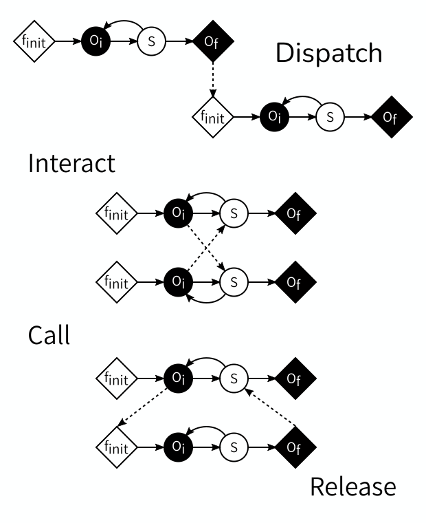
The three cases above demonstrate the four Coupling Templates defined by the MMSF. The first one, \(O_f\) to \(f_{init}\), is called dispatch. The second one, \(O_i\) to \(S\) is called interact, and usually comes in pairs. The third one and the fourth one usually go together, as the combination call (\(O_i\) to \(f_{init}\)) and release (\(O_f\) to \(S\)).

Given the constraints of which operators can send and which can receive, these are in fact all four possible types of connections, and between them they cover all kinds of temporal scale relations.

If the time domains or time scales overlap, but are not equivalent, then an additional component is needed that sits between the models; we will not go into that advanced use case here.

Spatial domains, scales and multiplicity

---

Having discussed temporal scales, let’s move on to the spatial scales. Like with scales in time, scales in space can be the same, overlap, be adjacent or be separated, and you can see which one you have by looking at your Scale Separation Map. Here’s another table with the interpretation of those relations in space:

Property	Relation	Description
Domain	Same	In the same place, acting on the exact same bit of reality
Domain	Overlap	Some parts in the same place, acting on the same bit of reality
Domain	Adjacent	Acting on two different bits of reality which touch each other (space)
Domain	Separated	Acting on two different bits of reality which do not touch (space)
Scale	Same	Same grain (dx) and extent (size)
Scale	Overlap	Grain or extent differs, but neither model has a grain larger than the extent of the other or an extent smaller than the grain of the other
Scale	Adjacent	One model’s extent equals the other’s grain
Scale	Separated	One model’s extent is smaller than the other model’s grain

Same spatial domain and scale

This is a very tight coupling, where usually the two processes end up in a single equation on the theory side, and in a single code in the implementation. Unless there is temporal scale separation, it’s probably better to combine the models into a single implementation. In case of temporal scale separation, a call-and-release template may be used and the state is passed back and forth between the models.

Same spatial domain, adjacent or separated scales

If one process is much smaller than the other, then the entire small process takes place within one grid cell or agent of the larger process. Frequently, this means that there are multiple instances of the smaller model, maybe even one for each grid cell or agent, with communication between the large-scale model and each small-scale model instance. Some kind of iterative equilibration between the models may be needed to reconcile the two representations of the state.

Adjacent spatial domains, same or overlapping spatial scales

If two processes are of similar size and resolution, but occur on adjacent domains, then they will each have their own state, and exchange boundary conditions. If there’s a temporal scale separation between them, then the call-and-release coupling template is used and the called (fast) model keeps its state in between calls.

Challenge 5: Spatial relations

Think of an example for each of the above spatial domain and scale relations. Can you think of examples that don’t fit any of them?

Example solution

• Reaction-diffusion models have the two processes acting on the same domain and spatial scale, but may be temporally scale-separated depending on parameter values.
• A crack propagation model coupling a continuum representation of a material sample to molecular mechanics models at specific points. Stresses and strains are exchanged in this case.
• In a simulation of In-Stent Restenosis, a complication of vascular surgery, a cell growth process in the wall of an artery is coupled with a fluid dynamics simulation of the blood flow through the artery. The domains are adjacent and boundary conditions are exchanged.

MMSL Diagrams

---

For larger coupled simulations consisting of several submodels and other components, drawing the complete submodel execution loop as we did above gets too complicated. Fortunately, a simplified notation is available in the form of the Multiscale Modelling and Simulation Language (MMSL). This language describes a coupled simulation as a set of components and the connections between them. Its YAML-based form, yMMSL, is used as the configuration language for MUSCLE3 (more on which in the next episodes). Its graphical form, gMMSL, provides a compact visual representation of a coupled model:

Coupling Templates in gMMSL

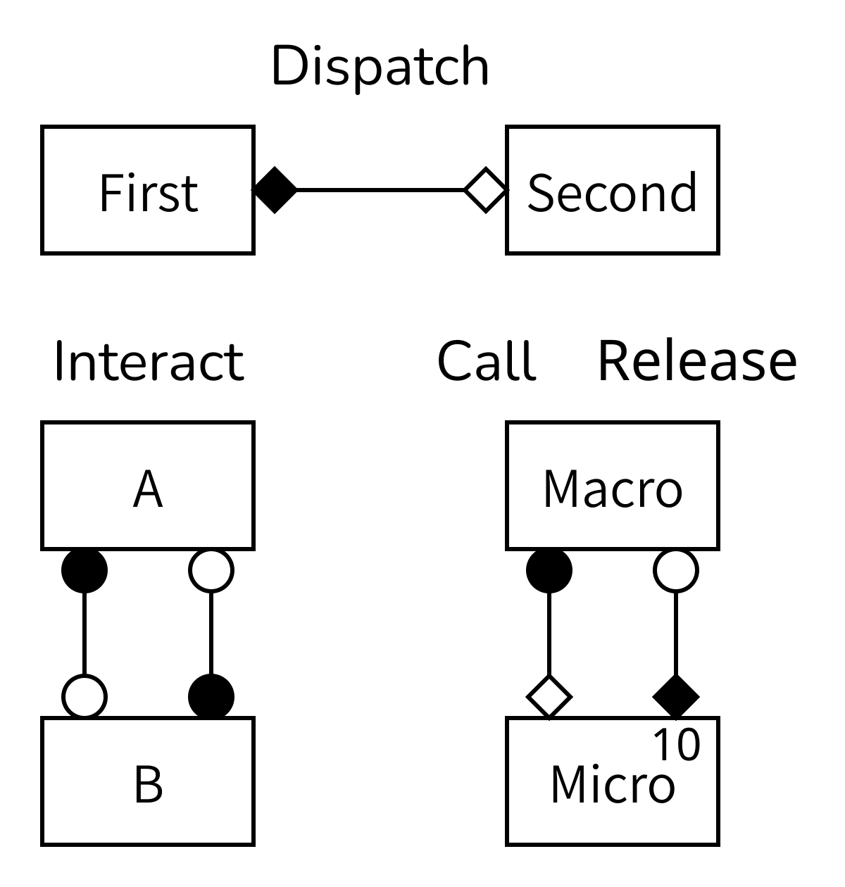
Challenge 6: Deciphering gMMSL

Explain the above figure.

Example solution

Each box represents a submodel. The lines show where information is sent from one model to another. The diamonds and circles designate the SEL operators that information is sent from and to. A number in the top right corner of a box is optional, but when it’s there it shows how many instances of that submodel exist. In this case, the model at the bottom right has temporal and spatial scale separation, so it uses the call-and-release coupling template and has multiple instances of the micromodel.

Note that there can be multiple lines or conduits between the same operators and models if multiple bits of information need to be transferred, but then these could also be glued together into a single message. This is a modelling decision, so do what works best for your model.

Not shown in the diagram is that the lines can be labeled with a label at each end showing the name of the port on the model that is being connected. Especially if there are multiple lines then it is necessary to do that to avoid confusion. More about this in the following episodes, when we connect two models using MUSCLE3.

Callout

Real simulations often need more than just the submodels, especially if you want to keep everything nice and modular. Different models often send and receive data in different formats for example, so that you need converters, and sometimes splitters and joiners that can split messages or join them together. If there is a scale difference, then some kind of scale bridge usually needs to be implemented, and for uncertainty quantification components may be needed that sample parameters and combine results into distributions.

These components are often simple functions, and can then be implemented just like a submodel with only an \(f_{init}\) and \(O_f\). Such a component can then be inserted in between a connection between two submodels by interrupting a conduit and putting it in between.

Key Points

• Physical processes take place on a domain and at certain scales in time and space
• Simulation models are described by the Submodel Execution Loop
• Given two models and their domains and scales, we can decide which coupling template to use to connect them
• An MMSL diagram can be used to visualise a complete coupled simulation

Content from MUSCLE3 - connecting a model to MUSCLE

---

Last updated on 2022-10-31 | Edit this page

Overview

Questions

• How do you connect an existing python model code to MUSCLE3?

Objectives

• Identify the inputs and outputs of your submodel and link them to ports
• Recognize the Submodel Execution Loop structure in your code
• Learn to connect a simple model to the MUSCLE3 library

Introduction

---

MUSCLE3 is the third incarnation of the Multiscale Coupling Library and Environment. MUSCLE and the MMSF were developed at the University of Amsterdam Computational Science Lab, and MUSCLE3 is the result of a collaboration with the Netherlands eScience Center. MUSCLE3’s purpose is to make creating coupled multiscale simulations easy. MUSCLE3 uses the Multiscale Modelling and Simulation Language (MMSL) to describe the structure of a multiscale model, and you will notice that the terminology in MUSCLE3 closely links to what you have learned in the previous episode about MMSF.

In this episode, we will be connecting a small model to MUSCLE3, so that we can connect it to a second model in the next episode.

Reaction-diffusion model

The example model for this course is a 1-dimensional reaction-diffusion model. This model models a 1-dimensional medium in which some chemical is constantly destroyed by a reaction, while it is also diffusing through the medium. A reaction submodel models exponential growth (or decline in this case, with a negative parameter) for each cell in the 1D grid. A diffusion submodel models diffusion through the 1D grid. This model is not very realistic, but we’re interested in the coupling, not in reaction-diffusion dynamics, so the simpler the better.

Reaction-diffusion models are a traditional example case for multiscale modelling because depending on the parameters used, they may be time-scale overlapping, adjacent or separated. In this example, we’re going to configure the diffusion model to be much slower than the reaction model, resulting in temporal scale separation.

To find out how to connect the models, we need to apply the MMSF to this particular situation. The reaction and diffusion processes act simultaneously on the same spatial and temporal domain. The discretisation of that domain in space is also the same for the two models, so that they have the same spatial scale. And there is temporal scale separation. According to the MMSF, that means that we have to use the Call-and-Release coupling template, with one instance of each submodel:

gMMSL diagram for the reaction-diffusion model

As you can see, each model will send and receive data on two operators, and we will connect them together as shown to form the full simulation.

MUSCLE3

Before we can create our coupled simulation however, we will need to connect each submodel to MUSCLE3. MUSCLE3 consist of three components:

libmuscle is a library that is used to connect component intances (e.g new or existing submodels) to a coupled simulation.

muscle_manager is the central manager of MUSCLE3 that starts up submodels and coordinates their interaction.

ymmsl-python is a Python library that contains class definitions to represent an MMSL model description. A yMMSL file serves as the interface between us (humans) and the muscle manager and is meant to describe the multiscale simulation and tell the muscle manager what to do.

Here, we will connect the reaction submodel (the micromodel) to the libmuscle library step by step. We’ll use yMMSL and the manager in the next episode.

Dissect your model

---

Open the file called reaction.py from the data folder that you downloaded in the setup section in a text editor. It contains a function called reaction that requires a numpy.array as input and returns another after doing some operations.

PYTHON

def reaction(initial_state: np.array) -> np.array:
    """
    ...
    """
    t_max = 2.469136e-6
    dt = 2.469136e-8
    k = -4.05e4

    U = initial_state.copy()

    t_cur = 0
    while t_cur + dt < t_max:
        U += k * U * dt
        t_cur += dt

    return U

The function starts with defining some parameters that are used for the calculations in the main while loop. The initial_state is copied to a new working state U before the simulation starts.

Why .copy()?

Instead of using .copy(), we could also just assign U to equal the initial state (e.g. U = initial_state). For this particular example it would not matter since we do not use initial_state anymore. But if we did that, we would change the contents of initial_state every time we do an operation on U, because both variables would point to the same object. Since the variable is called initial_state it would be very confusing if it would change during the model execution. When you want to expand or change the model later on, it can be dangerous if variables do not behave as their name suggests.

At every iteration of the loop, the state U is updated by adding a fraction of the old state, scaled by the parameter k and the size of a time step. Also the time counter t_cur is incremented with one time step. The while loop continues to run until t_cur has reached the value of the parameter t_max. Finally, when it exits the loop, the function returns the updated state U.

Challenge 1: Can you recognize the Submodel Execution Loop?

In the previous episode we have discussed the Submodel Execution Loop (SEL) and the various operators that are associated with it. In the code of the reaction function, can you recognize the beginning and end of the four operators (\(f_{init}\), \(O_i\), \(S\) and \(O_f\) ) plus the state update loop in this submodel? Mark these by placing the following 10 comments in the code:

• # begin F_INIT
• # end F_INIT
• # begin O_I
• # end O_I
• # begin S
• # end S
• # begin state_update_loop
• # end state_update_loop
• # begin O_F
• # end O_F

Show me the solution

PYTHON

def reaction(initial_state: np.array) -> np.array:
    """
    ...
    """
    # begin F_INIT
    t_max = 2.469136e-6
    dt = 2.469136e-8
    k = -4.05e4

    U = initial_state

    t_cur = 0
    # end F_INIT

    # begin state_update_loop
    while t_cur + dt < t_max:
        # begin O_I
        # end O_I

        # begin S
        U += k * U * dt
        t_cur += dt
        # end S
    # end state_update_loop

    # begin O_F
    return U
    # end O_F

\(f_{init}\) is where everything gets initialised, at the top of the function. This is not just the state, but also parameters and helper variables. Then, the Submodel Execution Loop specifies two operators within the state update loop. \(O_i\) comes before \(S\) and you can use it to send information to the outside world with (part of) the current state. \(O_i\) is empty here, because this original model didn’t produce any output for each state. It did update its state however, so that part of the code is in \(S\). Finally, returning a result falls under \(O_f\).

Creating an Instance object

---

To let a model communicate with the muscle manager, other submodels and the outside world, we need to create a libmuscle.Instance object. An instance is a running submodel, and the Instance object represents this particular instance to MUSCLE3:

PYTHON

from libmuscle import Instance
from ymmsl import Operator

def some_example_submodel():
    instance = Instance({
            Operator.F_INIT: ['initial_state_a', 'initial_state_b'],
            Operator.O_I: ['some_intermediate_state'],
            Operator.S: ['some_other_intermediate_state'],
            Operator.O_F: ['final_state_a', 'final_state_b']})

The constructor takes a single argument, a dictionary that maps ymmsl.Operator objects to lists of ports. Ports are used to communicate with other simulation components. They have a name, and they are associated with a Submodel Execution Loop operator, which determines whether they are input or output ports. The operator that they are mapped to determines how the port is used, as explained in the previous episode. The names of the available operators correspond to their theoretical counterparts (\(f_{init}\), \(O_i\), \(S\) and \(O_f\) ).

What ports do we need?

Question: In our example of the reaction submodel, what ports do we need to communicate the model state to the outside world? Come up with good names. What operators would we need to map them to?

Show me the solution

In this model, we need:

• a single input port that will receive an initial state (e.g. named “initial_state”) at the beginning of the model run and it should be mapped to the \(f_{init}\) operator
• a single output port that sends the final state (e.g. named “final_state”) at the end of the reaction simulation to the rest of the simulation, it should be mapped to the \(O_f\) operator

The reuse loop

---

In multiscale coupled simulations, submodels often have to run multiple times, for instance because they are used as a micro model or because they are part of an ensemble that cannot be completely parallelised. To make this possible, we will wrap the entire submodel in a loop, the so-called reuse loop. Exactly when this loop needs to end often depends on the behaviour of the whole model, and is not easy to determine in advance, but fortunately MUSCLE will do that for us if we call the Instance.reuse_instance() method.

PYTHON

    while instance.reuse_instance():
        # F_INIT
        # State update loop
        # O_F

Challenge 2: Creating an Instance and adding a loop

Add the following to our reaction model code:

• a libmuscle.Instance object with the appropriate operator-port dictionary
• the reuse loop

Show me the solution

PYTHON

from libmuscle import Instance
from ymmsl import Operator

def reaction(initial_state: np.array) -> np.array:
    """
    ...
    """
    instance = Instance({
            Operator.F_INIT: ['initial_state'],       # np.array
            Operator.O_F: ['final_state']})           # np.array

    while instance.reuse_instance():
        # begin F_INIT
        t_max = 2.469136e-6
        dt = 2.469136e-8
        k = -4.05e4

        U = initial_state

        t_cur = 0
        # end F_INIT

        # begin state_update_loop
        while t_cur + dt < t_max:
            # begin O_I
            # end O_I

            # begin S
            U += k * U * dt
            t_cur += dt
            # end S
        # end state_update_loop

        # begin O_F
        return U
        # end O_F

Note that the type of data that is sent is documented in a comment. This is obviously not required, but it makes life a lot easier if someone else needs to use the code or you haven’t looked at it for a while, so it’s highly recommended. MUSCLE3 does not require you to fix the type of the messages you’re sending to a port in advance; in principle you could send a different type of message every time you send something. The latter is a bad idea, but the flexibility makes development much easier.

Settings

---

Next is the first part of the model, in which the model is initialised. Nearly every model needs some settings that define how it behaves (e.g. the size of a timestep or model specific parameters). With MUSCLE, we can specify settings for each submodel in a central configuration file, and get those settings from libmuscle in the model code. This way, we don’t have to change our model code every time if we want to try a range of values (for instance, to perform a sensitivity analysis). We can use the Instance.get_setting function instead to ask the MUSCLE manager for the values. Putting the values in the configuration file will be covered in the next episode, here we’ll look at how to get them from libmuscle.

PYTHON

    some_variable = instance.get_setting('variable_name', 'variable_type')

Type checking

The second argument, which specifies the expected type, is optional. If it is given, MUSCLE will check that the user specified a value of the correct type, and if not raise an exception.

Challenge 3:

In our example, several settings have been hard-coded into the model:

• the total simulation time to run this sub-model, t_max
• the time step to use, dt
• and the model parameter, k

Change the code such that we request these settings from the MUSCLE manager.

Show me the solution

PYTHON

from libmuscle import Instance
from ymmsl import Operator

def reaction(initial_state: np.array) -> np.array:
    """
    ...
    """
    instance = Instance({
            Operator.F_INIT: ['initial_state'],       # np.array
            Operator.O_F: ['final_state']})           # np.array

    while instance.reuse_instance():
        # begin F_INIT
        t_max = instance.get_setting('t_max', 'float')
        dt = instance.get_setting('dt', 'float')
        k = instance.get_setting('k', 'float')

        U = initial_state

        t_cur = 0
        # end F_INIT

        # begin state_update_loop
        ...

Note that getting settings needs to happen within the reuse loop; doing it before can lead to incorrect results.

Receiving messages

---

Apart from settings, we can use the Instance.receive function to receive an initial state for this submodel on the initial_state port. Note that we have declared that port above, and declared it to be associated with the F_INIT operator. During F_INIT, messages can only be received, not sent, so that declaration makes initial_state a receiving port.

The message that we will receive can contain several pieces of information. For now, we are interested in the data and timestamp attributes. We assume the data to be a grid of floats containing our initial state and the time stamp tells us the simulated time at which this state is valid. We can receive a message and store the data and timestamp attributes in the following way:

PYTHON

    msg = instance.receive('initial_state')

    data = msg.data.array.copy()
    timestamp = msg.timestamp

Why .copy() again?

The msg.data attribute holds an object of type libmuscle.Grid, which holds a read-only NumPy array and optionally a list of index names. Here, we take the array and make a copy of it for data, so that we can modify data in our upcoming state update. Without calling .copy(), the variable data would end up pointing to the same read-only array, and we would get an error message if we tried to modify it.

The timestamp attribute is a double precision float containing the number of simulated (not wall-clock) seconds since the whole simulation started. Since t_cur is assigned the value of the timestamp, we don’t need to make a copy.

State update loop

---

The actual state update happens in the operator \(S\) in the Submodel Execution Loop and, in our example model, it is determined entirely by the current state. Since no information from outside is needed, we do not receive any messages, and in our libmuscle.Instance declaration above, we did not declare any ports associated with Operator.S.

The operator O_I provides for observations of intermediate states. In other words, here is where you can send a message to the outside world with (part of) the current state. In this case, the O_I operator is empty; we’re not sending anything.

One thing we need to be aware of is time. Most models depend on time in some way and it is good to be aware of the various time frames. Libmuscles messages support passing on timestamps to be able to keep track of the global simulation time of the coupled model. It is easier to keep track of only one time frame and it is therefore good practice to add the timestamp that accompanied the initial state to the sub-model simulation time steps instead of starting at zero for every sub-model instance.

Challenge 4: Receiving the initial state and keeping track of time

Where previously we had received initial_state from the function call, we now want to get it through a libmuscle message. Add statements to receive a message on the initial_state port and store the data and timestamp attributes in an appropriate place.

Also make sure the state update loop tracks global simulation time (corrected by the received timestamp).

Show me the solution

PYTHON

from libmuscle import Instance
from ymmsl import Operator

def reaction() -> np.array:
    """
    ...
    """
    instance = Instance({
            Operator.F_INIT: ['initial_state'],       # np.array
            Operator.O_F: ['final_state']})           # np.array

    while instance.reuse_instance():
        # begin F_INIT
        t_max = instance.get_setting('t_max', 'float')
        dt = instance.get_setting('dt', 'float')
        k = instance.get_setting('k', 'float')

        msg = instance.receive('initial_state')
        U = msg.data.array.copy()

        t_cur = msg.timestamp
        t_max = msg.timestamp + t_max
        # end F_INIT

        # begin state_update_loop
        while t_cur + dt < t_max:
        ...

Time keeping

Both t_cur and t_max used to be relative to the start of the submodel, but now represent absolute simulation time of the coupled system. The length of the while loop will not change, but in this way we would be able to send out the current global simulation time t_cur in the state update loop using the I_O operator. It is also possible to keep t_cur and t_max relative to the start of the submodel and only correct for the received global timestamp when you send out a message. It is often however preferable to keep track of only one single timeframe and make the corrections right at the receiving end.

Sending messages

---

To send a message we first have to construct a libmuscle.Message object containing the current simulation time and the current state. We will convert the numpy.array to a libmuscle.Grid object first.

MUSCLE grids

We convert our numpy.array explicitly into a libmuscle.Grid object, so that we can add the name of the dimensions. In our example case there is only one, and “x” is not very descriptive, so we could have also passed the array directly, in which case MUSCLE would have done the conversion for us and sent a libmuscle.Grid without index names automatically.

The optional second parameter is a second timestamp, which is only used in more advanced applications and can be set to None here.

PYTHON

from libmuscle import Grid, Message
my_message = Message(my_timestamp, None, Grid(my_state, ['x']))

To send the message, we specify the port on which to send, which needs to match the name of a port specified when we created the Instance object:

PYTHON

instance.send('final_state', final_message)

Challenge 5: Send back the result

In the \(O_f\) operator of your model construct a message and replace the return statement with a call to libmuscle.Instance.send() to send the final state to the outside world.

Show me the solution

PYTHON

from libmuscle import Instance, Grid, Message
from ymmsl import Operator

def reaction():
    """
    ...
    """
    instance = Instance({
            Operator.F_INIT: ['initial_state'],       # np.array
            Operator.O_F: ['final_state']})           # np.array

    while instance.reuse_instance():
        # begin F_INIT
        t_max = instance.get_setting('t_max', 'float')
        dt = instance.get_setting('dt', 'float')
        k = instance.get_setting('k', 'float')

        msg = instance.receive('initial_state')
        U = msg.data.array.copy()

        t_cur = msg.timestamp
        t_max = msg.timestamp + t_max
        # end F_INIT

        # begin state_update_loop
        while t_cur + dt < t_max:
            # begin O_I
            # end O_I

            # begin S
            U += k * U * dt
            t_cur += dt
            # end S
        # end state_update_loop

        # begin O_F
        final_message = Message(t_cur, None, Grid(U, ['x']))
        instance.send('final_state', final_message)
        # end O_F

Right now your sub-model is ready to be used by the muscle manager. We will couple it to another submodel and configure it to run the coupled simulation in the next chapter.

Key Points

• MUSCLE3 implements the MMSF theory, using the same terminology and MMSL for configuration of the coupled simulation
• First analyze your code to find the Submodel Execution Loop structure
• MUSCLE lets the submodels communicate through messages, containing model states and simulation times

Content from MUSCLE3 - coupling and running

---

Last updated on 2022-10-31 | Edit this page

Overview

Questions

• How do you couple multiple sub-models using MUSCLE3?
• How do you run a coupled simulation with MUSCLE3?

Objectives

• Demonstrate how MUSCLE3 implements the Multiscale Modelling and Simulation Language (MMSL)
• Configure a coupled simulation with MUSCLE3
• Run a coupled simulation using MUSCLE3

Introduction

---

We managed to connect one of our sub-models, the reaction model, to MUSCLE. In order to make a coupled simulation, we need at least two models. The second model here is the diffusion model. We prepared it for you, adding the necessary MUSCLE bindings and comments similar to what we did for the reaction model. You can open it from diffusion.py.

Investigating the macro model

---

Challenge 1: Investigating the diffusion model

The diffusion.py file contains a couple of functions, as well as a few lines of code that may come in useful later. For now, let’s focus on the diffusion function.

• Compared to the reaction function you made previously, what is different, other than the mathematics of the model itself?

Show me the solution

• The ports are named differently, and are attached to different operators
• The send and receive statements are now within the state update loop

Connecting the models together

---

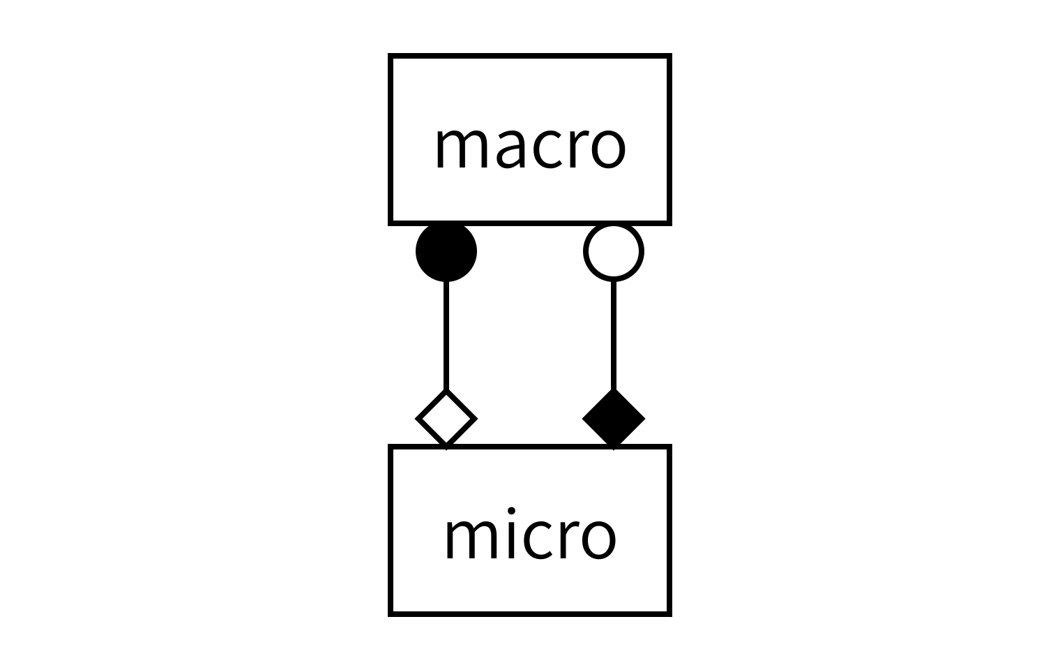
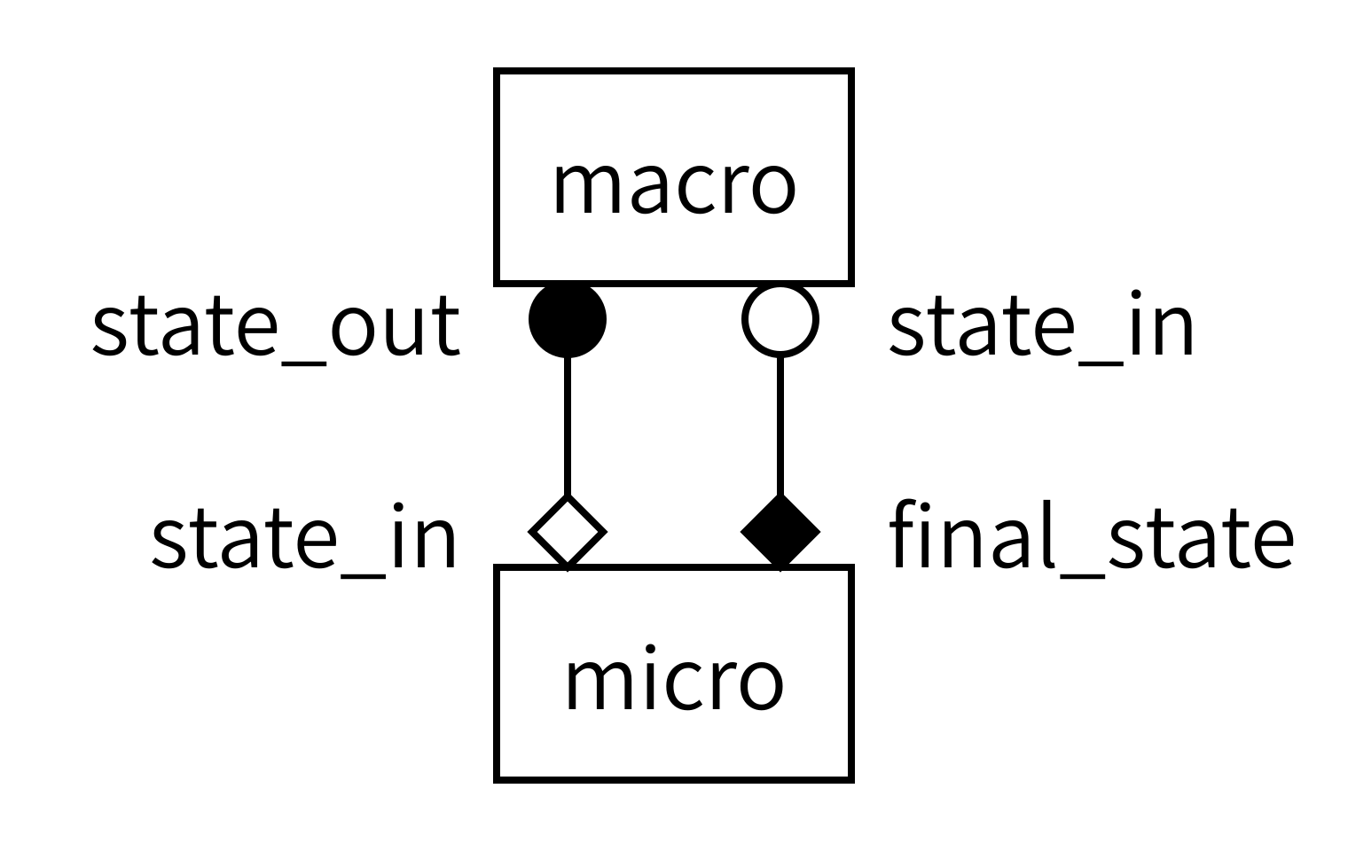
With both models defined, we now need to instruct MUSCLE3 on how to connect them together. Recall the gMMSL diagram from the previous episode (with port names, this time):

gMMSL diagram for the reaction-diffusion model

Since diagrams aren’t valid Python, we need an alternative way of describing this model in our code. For this, we will create a MUSCLE configuration file written in the yMMSL language. This file tells the MUSCLE manager about the existence of each submodel and how it should be connected to the other components.

Challenge 2: Creating the yMMSL file

Open the file reaction_diffusion.ymmsl. In it, you’ll find an incomplete yMMSL description of the coupled simulation, as shown below. Your challenge? Complete it!

Tip: remember that this is a textual description of the diagram above. All the information you need is in there.

YAML

ymmsl_version: v0.1

model:
  name: reaction_diffusion

  components:
    macro:
      implementation: diffusion
      ports:
        o_i: state_out
        ...

    ...
      implementation: reaction
      ...

  conduits:
    macro.state_out: micro.initial_state
    ...

Show me the solution

YAML

ymmsl_version: v0.1

model:
  name: reaction_diffusion_python

  components:
    macro:
      implementation: diffusion
      ports:
        o_i: state_out
        s: state_in

    micro:
      implementation: reaction
      ports:
        f_init: initial_state
        o_f: final_state

  conduits:
    macro.state_out: micro.initial_state
    micro.final_state: macro.state_in

First, we describe the two components in this model. Components can be submodels, or helper components that convert data, control the simulation, or otherwise implement required non-model functionality. The name of a component is used by MUSCLE as an address for communication between the models. The implementation name is intended for use by a launcher, which would start the corresponding program to create an instance of a component. It is these instances that form the actual running simulation. In this example, we have two submodels: one named macro and one named micro. Macro is implemented by an implementation named diffusion, while micro is implemented by an implementation named reaction.

Second, we need to connect the components together. This is done by conduits, which have a sender and a receiver. Here, we connect sending port state_out on component macro to receiving port initial_state on component micro.

Adding settings

---

The above specifies which submodels we have and how they are connected together. Next, we need to configure them by adding the settings to the yMMSL file. These will be passed to the models, who get them using the Instance.get_settings() function. Go ahead and add them to your reaction_diffusion.ymmsl:

YAML

settings:
  micro.t_max: 2.469136e-6
  micro.dt: 2.469136e-8
  macro.t_max: 1.234568e-4
  macro.dt: 2.469136e-6
  x_max: 1.01
  dx: 0.01
  k: -4.05e4    # reaction parameter
  d: 4.05e-2    # diffusion parameter

Look at the names of the settings. Does anything stand out to you?

Specifying resources

---

Finally, we need to tell MUSCLE3 whether and if so how each model is parallelised, so that it can reserve adequate resources for each component. In this case, the models are single-threaded so that is what we specify. Again, add this to your file.

YAML

resources:
  macro:
    threads: 1
  micro:
    threads: 1

Note that we specify resources for each component, not for each implementation.

Launching the simulation

---

This gives us all the pieces needed to construct a coupled simulation. All we need is the two model functions and the configuration, then we can connect them together and run the whole thing. The model functions we can import from the files we saw before:

PYTHON

from diffusion import diffusion
from reaction import reaction

To load the configuration, we use the load() function from the ymmsl module that comes with MUSCLE3:

PYTHON

from pathlib import Path
import ymmsl

configuration = ymmsl.load(Path('reaction_diffusion.ymmsl'))

Finally, we need to create a connection from the names of the implementations listed in the yMMSL file to the Python functions that are those implementations:

PYTHON

implementations = {'reaction': reaction, 'diffusion': diffusion}

And then we can ask MUSCLE3 to start the coupled simulation:

PYTHON

from libmuscle.runner import run_simulation.

run_simulation(configuration, implementations)

You will find a coupled_model.py file with the others, which implements the above. It also configures Python’s logging subsystem to give us a bit more log output.

Challenge 3: Running the coupled simulation

If you haven’t already done so, add the settings and resources to your reaction_diffusion.ymmsl. Then, have a look at the coupled_model.py script and see if you can run it. It should show a plot on the screen showing the concentration over time. If not, try to find the problem! You should have a muscle_manager.log file, and maybe a muscle3.micro.log and muscle3.macro.log to help you figure out what went wrong.

Show me the solution

$ python3 coupled_model.py

Running separate programs using the MUSCLE3 manager

---

The above coupled_model.py script imports the models as Python functions, and then starts them using MUSCLE3’s runner.run_simulation() function. This works great for models consisting entirely of Python components, and which are small enough to run on the local machine. However, models written in other languages like C++ or Fortran cannot be imported as Python functions, and larger simulations may need to run on many nodes on an HPC cluster. For such simulations, we cannot use run_simulation(), and we need to use the MUSCLE3 manager instead.

The MUSCLE3 manager, like the runner, gets a model description and a list of implementations to use, and then starts each required instance by starting its implementation. That’s a fair bit of new terminology, so here is what those words mean:

Component

Represents a simulated process with a domain and a scale, or is a helper component. One box in the gMMSL diagram. May have a single instance, or multiple instances e.g. in case of spatial scale separation or if it’s part of a UQ ensemble.

Instance

A running program simulating a particular component. This may be a parallel program running on many cores or across many machines, or in could be a simple Python script.

Implementation

A computer program (e.g. a Python script) that can be started to create an instance.

Challenge 4: Running using the manager

In this final challenge, we’ll run the reaction-diffusion model using the MUSCLE3 manager. This takes three steps: turning the reaction model into a stand-alone program, telling the manager how to start the programs, and finally running it all.

Create a stand-alone Python program

First, you need to turn reaction.py into a stand-alone Python program.

Hint: Look at diffusion.py, which is already set up to do this. You can copy-paste and adapt from there.

Add an implementations section

Next, you need to add an implementations: section to your yMMSL file. The implementations section describes which implementations are available to run. Here’s a template for a Python program:

implementations:
  <implementation_name>:
    virtual_env: <absolute path to virtual env to load>
    executable: python
    args: <absolute path to Python script>

Add this section to your reaction_diffusion.ymmsl, and replace all the items in angle brackets with the correct values.

Run the simulation

To run the simulation using the manager, open a terminal and activate the virtual environment in which you’ve installed MUSCLE3. You can then start the simulation using muscle_manager --start-all reaction_diffusion.ymmsl. Do that, and inspect the output!

Show me the solution

To turn reaction.py into a stand-alone program, you need to add the final section of diffusion.py to the end, slightly modified:

if __name__ == '__main__':
    logging.basicConfig()
    logging.getLogger().setLevel(logging.INFO)
    reaction()

The yMMSL file then gets an implementations section like this:

implementations:
  reaction:
    virtual_env: /path/to/workdir/env
    executable: python
    args: /path/to/workdir/reaction.py

  diffusion:
    virtual_env: /path/to/workdir/env
    executable: python
    args: /path/to/workdir/diffusion.py

Then, you can run using

(env) $ muscle_manager --start-all reaction_diffusion.ymmsl

And that will create a directory named run_reaction_diffusion_<date>_<time> with all the log files and model output neatly organised.

Key Points

• Models may differ in which ports they have and when they send and receive
• The yMMSL file discribes components, conduits, settings and resources
• Running the coupled simulation can be done from a Python script
• For larger simulations and C++ and Fortran, submodels run as separate programs via the MUSCLE3 manager